
Previously in this series: Elementary Infra-Bayesianism1. There’s this paperEarlier last week I got nerd-sniped by a paper called Condensation: a theory of concepts (Eisenstat 2025). It’s the kind of paper where the abstract makes a claim so clean you assume you must be misreading it: roughly, there is a right answer to “what are the concepts in this data,” and any two agents who carve it up well enough will agree on what those concepts are.[1]If that sounds like John Wentworth’s natural abstractions hypothesis, yes, the family resemblance is strong. I wrote about something adjacent a while back. Condensation is a different formalization, but the punchline rhymes: structure in the data constrains what any good representation can look like. People on LessWrong seem to dig it, and I wanted to see what the fuss was about.The paper is forty pages of math and gives you no algorithm; it tells you what a good carving looks like, not how to find one. I spent a slightly embarrassing amount of time trying to get the basic objects to do something on a computer. This post is how far I got.[2]2. Concepts, scopes, and a scoreSay you observe three tokens[3]: cat dog catI’ll define a concept as a piece of information about that data.[4] “The topic is animals” is a concept. “Token 2 is dog, not cat” is also a concept. Concepts can come with a scope: the set of tokens a concept is about. The topic concept has scope {1,2,3}, because knowing the topic tells you something about all three tokens. The “token 2 is dog” concept has scope {2}, because it’s only about token 2.A representation is a list of (concept, scope) pairs. With three tokens there are seven possible scopes ({1}, {2}, {3}, {1,2}, {1,3}, {2,3}, {1,2,3}); a typical representation puts something at a few of them and leaves the rest empty.[5] Which scopes get concepts is the structure the theory cares about.One rule that representations need to satisfy for us to care about them: from the concepts whose scope includes token , you must be able to rebuild token . No information goes missing. (If you only filed “topic = animals” and nothing else, you couldn’t rebuild cat vs dog; that representation is invalid.)The star of this show, condensation, then gives you a score function that measures how efficient a representation is. It works like this: someone asks “tell me everything relevant to tokens {1,2}.” You answer by reading every concept whose scope overlaps {1,2}. In our example that’s the topic (scope {1,2,3}, overlaps), id (scope {1}, overlaps), and id (scope {2}, overlaps), but not id (scope {3}, no overlap). is the total bits you had to read.[6] You want small for every possible question; never read a concept that isn’t relevant, never read the same information twice.Three tokens (cat, dog, cat), four concepts filed at their scopes. A query about tokens {1,2} reads every concept whose scope overlaps {1,2}: the topic (scope {1,2,3}), id (scope {1}), and id (scope {2}), but not id (scope {3}).As I said up top, the paper doesn’t tell you how to find a good representation. The main theorem (4.15) says that any two representations that score well enough will end up filing roughly the same concepts at roughly the same scopes,[7] which is the sense in which concepts are “out there.”3. The same three tokens, three representationsLet me make that concrete with a small example that still has all the structure we care about.The data: a fair coin picks a topic, animals or tools, and then each of three tokens is independently one of two words from that topic (cat/dog or hammer/saw). There are four bits of information total: one topic bit (shared across all three tokens) and three token-identity bits (private to one token each). Here are some example draws:token 1token 2token 3topiccatdogcatanimalshammersawhammertoolsdogdogdoganimalssawhammersawtoolsThree representations of the same data:Trivial. Don’t bother finding shared concepts. File each raw token at its own scope.scopeconceptbits{1}id₁2{2}id₂2{3}id₃2Ask about tokens 1 and 2: you read 4 bits, but the true joint information is only 3 bits because they share a topic.[8] The topic bit is sitting inside both raw tokens, and you read it twice. Every multi-token question overpays.Oracle. File the topic at {1,2,3} and each token-identity bit at its singleton.scopeconceptbits{1,2,3}topic1{1}id₁1{2}id₂1{3}id₃1Every question costs exactly its entropy, which is the best you can do.Misfiled. Same four concepts as the oracle, but topic at scope {2,3} instead of {1,2,3}.scopeconceptbits{2,3}topic1{1}full token₁[9]2{2}id₂1{3}id₃1Ask about tokens 1 and 2: full token₁ (2 bits) + topic (1 bit) + id₂ (1 bit) = 4. The topic is in there twice, and you pay for both copies. for each of the seven possible queries . Oracle is flat at zero; misfiling lights up exactly the queries that span both copies of the topic bit.So the score does what you’d hope: lowest when each shared concept sits at exactly the scope it’s about, and it tells you which queries overpay when one doesn’t.We built all of these by hand, so nothing deep is happening yet. The question is whether a representation constructed from the activations of a neural network looks more like the oracle or the trivial one.4. A model gives you concepts; scope is your problemNow suppose the concepts come out of a language model like GPT-2 or Claude rather than being hand-built.I trained a tiny 4-layer transformer on the three-token topic data from §3. A single weighted sum of the residual stream (the running vector that each layer reads from and writes to) recovers the topic with perfect accuracy:Tokens go through a tiny 4-layer LM; a linear probe on the residual stream recovers the topic (“animals”) with 100% accuracy. The concept is there; the question is what scope to assign it.So the model has learned the right concept. The question is: what scope do we assign it?One naive answer is “the feature’s scope is all the tokens the model has seen so far,” since that’s what the activation depends on. But that gives the same answer for every feature, so it can’t distinguish a feature about one token from a feature about the whole sequence.[10]A better method here is mutual information: scope = the set of tokens the feature is correlated with. The topic is correlated with all three tokens (each token’s first bit is the topic), so MI says scope {1,2,3}, which is the oracle representation from §3. The score goes to zero.[11]At scale, the standard way to get candidate concepts out of a language model is a sparse autoencoder (SAE): you learn a large set of directions in the residual stream such that, for any given input, only a few of them are active. Each direction is called a feature, and the hope is that “feature k is on” means something interpretable: this is about cooking, there’s an open bracket, the subject is plural. An SAE gives you features, but it does not give you their scopes, so you still need a method like MI to tag each one.5. Does it work on real models?The three-token toy was reassuring, but it was four bits of hand-built data. The question that matters is whether the score does anything useful when the concepts come out of an actual language model on actual text. To find out, I wanted to carefully expand the domain of the experiment along two axes: model size (from a tiny 4-layer transformer up to GPT-2 small) and dataset complexity (from planted ground truth up to real text).The pipelineTake 50,000 windows of text, tokens each.Run each through a language model and read the residual stream at the last token (by then the model has seen all ).Decompose those vectors three ways: an SAE, PCA (the textbook find-the-biggest-directions method), and random projections (the control: directions that mean nothing). Each gives you a few hundred features.Turn each feature into a concept: pick a threshold so the feature is ON for the top % of windows and OFF for the rest.[12] Tag it with a scope by MI, the set of token positions it’s correlated with. Keep the top most informative.Compute . Report : how many bits better (or worse) than the trivial representation from §3 that just stores each token raw. Negative means the method found shared concepts that actually save bits.[13]I sweep the threshold in step 4 and report each method’s minimum , letting the score pick its own threshold.[14] The other knobs in steps 1–4 I either swept or held fixed, and the thing I’m reporting throughout is the ordering (SAE vs PCA vs random), which survived every knob I turned.[15] The aggregate number is shakier (there’s a weighting choice in step 5 that can shift it) so don’t read any single number as a constant of nature.The datasetsA planted toy where I know the ground truth. Eight tokens, with seven planted shared concepts arranged in a binary tree: one about all eight tokens, one about tokens 1–4, one about 5–8, and one about each adjacent pair (1–2, 3–4, 5–6, 7–8). Each is a yes/no flag that’s “yes” 15% of the time. I pack them into six dimensions so they overlap a little and the SAE has to actually un-mix them.[16] Some example sequences:tok 1tok 2tok 3tok 4tok 5tok 6tok 7tok 8active flags0.31−0.420.87−0.150.63−0.290.44−0.71global, pair₃₄−0.550.12−0.330.68−0.210.45−0.620.19half₅₋₈, pair₇₈The oracle representation (true concepts at true scopes) scores .TinyStories. 50,000 eight-word openings from children’s stories. The positional structure here is real: “once upon a time there was a” lives at positions 1–7, and it’s the most common pattern by far. I ran this with both a small 4-layer transformer and GPT-2 small.sentence openingonce upon a time there was a littleone day a girl named lily went tothe sun was shining and the birds weretom and his mom went to the parkInduction. A setting designed to have one very specific shared concept. The prompt is something like cat dog bird fish bee cat ___where five random words are followed by a repeat of word 1, and the model should complete with word 2. GPT-2 small gets this right 75% of the time. I read the residual stream at the repeat (token 6), where the model has just recognised “that’s cat again.” The shared concept the features should pick up is “word 1 = cat,” scope {1,6}: it’s about token 1 (where cat first appears) and token 6 (where it appears again). The words come from a fixed pool of 50.ResultsOn the planted toy, the SAE recovers most of the ground truth: it gets 86% of the way to the oracle score, and the threshold at which it scores best is 15%, which is exactly the true rate the concepts were generated at. The score found the right threshold without being told it. PCA and random projections both fall well short.[17]On TinyStories, the ordering holds: SAE outperforms PCA, which outperforms random. The gaps are smaller than the toy (real text has less clean shared structure than seven planted flags), but consistent across both the small model and GPT-2 small. The SAE’s top feature fires on “once upon a time there was a”: one yes/no concept that tells you something about all eight tokens at once. PCA’s top feature fires on whether the last token is a function word: a concept about one token.[18]On induction, PCA wins, and not by a little.In the toy panel, the SAE’s best score sits at the true 15% rate and nearly touches the oracle line. In the induction panel, PCA’s curve keeps falling while SAE’s turns back up.Why PCA wins on inductionI want to dwell on this, because my prior was “SAE beats PCA” and the score disagreed. The shared concept is “which of 50 words is word 1,” not a yes/no flag but a 50-way choice worth bits. With four binary concepts to spend on encoding that choice, the SAE spends them on near-one-hots: its top features are literally “word 1 = gym,” “word 1 = pen,” “word 1 = fan,” “word 1 = cup,” each precise about 2% of inputs and silent on the other 98%. PCA spends its four concepts on coarse splits, each one ON for roughly 20% of the pool, vague about everything but covering all of it. Four coarse bits encode more of a 50-way variable than four one-hots do; the score is reporting that correctly. Shrink the pool to 8 words and PCA’s lead shrinks proportionally, confirming it’s the cardinality of the underlying variable that matters.[19] [20]6. How far I got, and what worries meThis is how far I got. The score does something: it distinguishes SAE from PCA from random in the right direction on controlled data, it finds ground-truth thresholds without being told, and it delivers at least one genuinely surprising result (PCA beating SAE on induction). But I want to be clear-eyed about what this is and isn’t.In this setting, the condensation score measures whether a decomposition’s inductive bias matches the structure of the shared concepts in the data. SAEs assume shared concepts are rare yes/no flags, PCA doesn’t assume that. So when the shared concepts are rare yes/no flags (the toy, TinyStories), SAE wins and when the shared concept is a 50-way categorical (induction), PCA wins. When there’s nothing shared, or the model never computed it, neither beats trivial.A few things I think this buys you, if it holds up:Scope is half the concept. Interpretability mostly treats a “concept” as a direction in activation space, full stop. Condensation says it’s a (concept, scope) pair, and §4 showed that scope assignment is a real choice and there’s an opinionated score that allows us to compare choices. “This feature means ” and “this feature is about tokens through ” are different claims, and circuits work tends to slide between them without noticing.Feature splitting has a signature. When an SAE breaks one underlying variable into many features, those features all land at the same scope, and penalizes exactly that (you read concepts where one would do). At scale, an SAE’s known split-feature families should show up as scope collisions, and a decomposition that merges them should score better. That’s a testable prediction.You could use this to choose decomposition methods per-circuit. Different parts of the same model plausibly have different kinds of shared concepts: induction is a categorical choice since “is this Python” is a yes/no flag. The score gives you a per-circuit reason to pick the decomposition rather than committing to SAEs everywhere, which is roughly where the SAEs-are-disappointing discourse has been heading anyway. And nothing here is SAE-specific; the pipeline takes any features-from-activations method.The theory is beautiful, and I have a lot of research ideas for how to fill in some of the implementation details:A principled algorithm for scope assignment would be awesome. I used MI because it worked on the toy, which is not a great justification. Turning concepts extracted from an SAE/from PCA into something that allows us to compute mutual information is tricky. Binarizing features throws away most of their information, and quantizing gets kind of messy.The number of possible scopes doubles with every token, so past a certain you can’t check them all.[21]And I’m not confident that the pipeline choices that work at will survive at , or that the orderings I’m seeing on 50,000 windows will hold at 500,000.That’s a lot of open questions before this approach would be ready for crunch-time deployment.[22]But the biggest gap is that I have not tested the paper’s actual theorem: that two good-scoring representations agree on what concepts they find. Everything above is “here’s a new scoring function for decomposition methods, and it gives sensible rankings.” That’s useful, but it’s an eval metric, not evidence that concepts are real. Condensation’s claim is stronger: any two representations that score well enough should converge on the same (concept, scope) pairs, and that’s what would make this about natural abstractions rather than about SAEs. Testing this could be relatively straightforward: train two SAEs with different seeds, extract their top concepts, and see whether χ agreement (Theorem 5.8) actually holds. I might do that in a follow-up, but I wanted to publish this much first, because I think more people poking at this independently is more valuable than me polishing in private.^Theorem 4.15, if you want to look it up. The actual statement is about amalgamations of latent variable models and is considerably more hedged than my gloss.^Most of the code was written by Claude in a long pair-programming session, which is the way things go these days. The mistakes in interpretation are mine.^Note that ‘tokens’ here is a choice I’m making, not something the theory demands. Scopes are defined over whatever observations you pick: token positions, syntactic constituents, document sections. Different choices give different possible scopes and a different theory of what the concepts are about.^A note on terminology: in the paper, a “concept” is technically the full (concept, scope) pair, not just the piece of information. I’m using “concept” more loosely to mean the piece of information itself, and “scope” separately, because that matches how most people in interpretability already think about features. The distinction only matters when you read the theorems.^The paper calls the concepts (latent variables, indexed by their scope ) and the whole collection a “latent variable model.” I’m going to keep saying “concepts” and “scopes” because the moment I write my eyes glaze over, and I start writing footnotes.^“Bits” throughout means information-theoretic bits: the entropy of a variable is how many bits, on average, it takes to write down its value. A fair coin is 1 bit. A fair 50-sided die is bits.^Theorem 4.15. The agreement is “cumulative”: the information at-and-above any scope matches, even if two representations distribute it across the levels differently. There’s an approximate version (5.8) for representations that score well but not perfectly, which is the one that matters in practice.^Why two bits each? Each token is one of four words (two topics × two words), uniform, so .^The rebuild rule forces this: {1}’s concepts have to be enough to reconstruct token 1, and “id₁” alone doesn’t cut it without the topic. So {1} stores the full token (2 bits, topic baked in).^You could also train the SAE on all possible truncations of each context and check whether a feature appears at each truncation length. This would give fine-grained scope information but is expensive; I didn’t try it. The mechanistic interpretability community has mostly focused on attributing features to predictions rather than to input tokens, using techniques like attribution patching (Nanda 2023) or circuit tracing (Anthropic 2025). These are closer in spirit to the attribution method than to MI.^People noticed the SAE connection in the comments on Demski’s post. As far as I know nobody’s actually computed the score before; that’s what the rest of this post does.^The threshold is essentially a choice of firing rate in a rate-coding scheme: above what activation level does a feature count as “on”? The analogy to spike-rate coding in neuroscience is not exact, but the tradeoff (too high and you lose signal, too low and everything fires) is the same.^The best possible (what the oracle gets) equals minus the total correlation of the tokens, i.e., how many bits of shared information exist across them. This isn’t a new quantity; what’s new is that the scope structure determines how close a given representation gets to it, and §3 showed that filing the right concept at the wrong scope falls short.^The threshold matters: too high and every concept is a coin flip, too low and every concept is a constant. Sweeping and reporting the minimum turned out to be the fix that made the comparison stable, after I’d spent a while fooling myself with a fixed threshold.^There are roughly a dozen choices in this pipeline and I won’t pretend they’re all principled. One aspect worth highlighting: each token is also stored raw at its own scope (so the rebuild rule is always satisfied, but it means most of is the raw tokens and the features are a perturbation on top).^Six dimensions, seven concepts: each concept is a random binary vector in , and each token is the sum of the concept vectors for the flags that are on, plus Gaussian noise. This forces overlap between the concepts in the observed dimensions, so the SAE has to un-mix them rather than just reading them off separate coordinates.^I also ran three settings where the answer should be “nobody wins”: random 12-token windows from the open web (no slot-aligned structure for anyone to find), a templated dataset with independent slot-fills (structure, but none of it shared across positions), and two-digit addition (GPT-2 can’t add, so the carry bit isn’t in the residual to be found). All three null out, with every method within ~0.1 bits of trivial. The open-web null is worth being careful about: it doesn’t mean “real text has no shared concepts,” just that it has no concepts shared across token positions in a random window. “Token position” was a choice I made in step 1, not something the theory handed down. The TinyStories results work because sentence-aligned openings have positional structure. A different choice of what the are (syntactic constituents, say, instead of positional slots) is probably what it’d take to get traction on open text.^I checked these aren’t just me squinting: standard auto-interp protocol (show an LLM 12 examples, ask for a one-line explanation, score whether the explanation predicts held-out examples). Mean balanced accuracy over the top-8 features: SAE 0.62 ± 0.18 (the “once upon a time” feature alone scores 0.95), PCA 0.55 ± 0.05, ICA and random ~0.52. Chance is 0.50. is small; the SAE-vs-rest gap is about one SAE-std.^You could read this as “you starved the SAE, give it 50 features and it’d win.” Maybe. But there’s a condensation-native reading I like better: the theory wants one concept at scope {1,6}, and the SAE shatters it into fifty features all at the same scope, feature splitting.^This result also convinced me the score isn’t circular. The worry: scope is defined as “tokens the feature is correlated with,” and rewards features correlated with many tokens, so of course high-MI methods win. But here every method is scoped by the same MI rule, the SAE’s features are not lower-MI than PCA’s, and the SAE still loses. What responds to isn’t “did you find correlated features” but whether the shape of the feature (yes/no flag vs. one-of-) matches the shape of the shared concept it’s supposed to encode.^One fun thing to think about here is whether oldschool computational linguistic style tagging of *syntactic constituents* (noun phrases, verb phrases, clauses) might usefully constrain the power set to something tractable. Scoring only syntactic constituents, or weighting by a parse tree, would make $N$=50 tractable and would be a fun thing to be wrong about.^Also untouched: using as a training objective instead of an eval. The let-the-score-pick-its-threshold trick suggests you’d be jointly learning features and their discretization, which sounds either elegant or completely cursed.^Attribution (Meng et al. 2022, Heimersheim 2024): delete the topic feature, and predictions for tokens 2 and 3 get worse (the model was using topic to narrow them down), but the prediction for token 1 doesn’t change (token 1 is predicted from nothing, before topic is known). The reason is structural: in an autoregressive model, the topic doesn’t exist until token 1 has been read, so the model can’t use it to predict token 1, so attribution can’t see that it’s about token 1. This gives the misfiled representation from §3, and the score overpays at exactly the queries you’d expect.^Attribution and MI aren’t even two estimators of the same thing; they’re different questions. Attribution asks “which predictions does this concept affect”; MI asks “which tokens is this concept about.” If you care about the model’s behaviour, attribution is right; if you care about the data’s structure, MI is. Condensation as written is about the data.Discuss Read More
Elementary Condensation
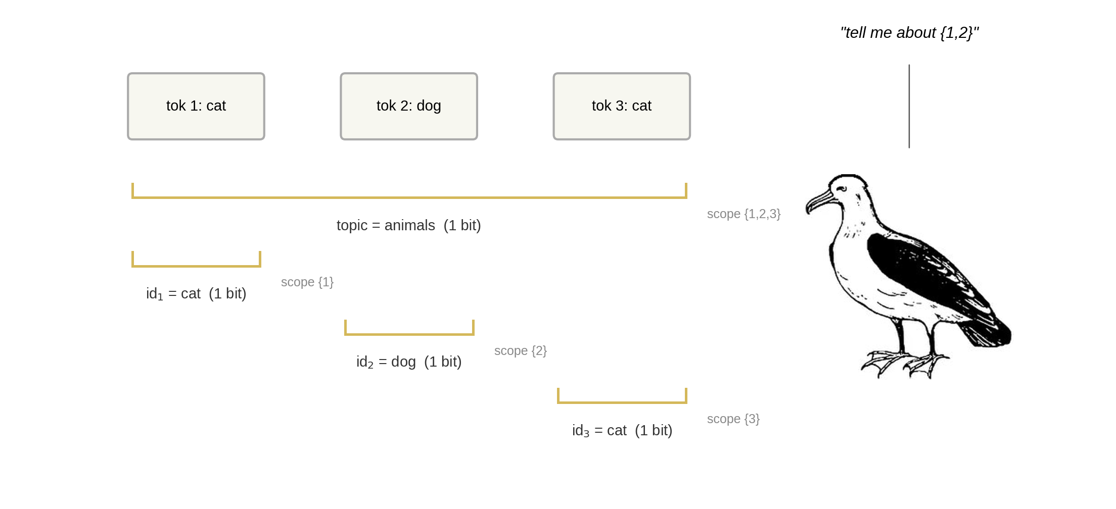
Previously in this series: Elementary Infra-Bayesianism1. There’s this paperEarlier last week I got nerd-sniped by a paper called Condensation: a theory of concepts (Eisenstat 2025). It’s the kind of paper where the abstract makes a claim so clean you assume you must be misreading it: roughly, there is a right answer to “what are the concepts in this data,” and any two agents who carve it up well enough will agree on what those concepts are.[1]If that sounds like John Wentworth’s natural abstractions hypothesis, yes, the family resemblance is strong. I wrote about something adjacent a while back. Condensation is a different formalization, but the punchline rhymes: structure in the data constrains what any good representation can look like. People on LessWrong seem to dig it, and I wanted to see what the fuss was about.The paper is forty pages of math and gives you no algorithm; it tells you what a good carving looks like, not how to find one. I spent a slightly embarrassing amount of time trying to get the basic objects to do something on a computer. This post is how far I got.[2]2. Concepts, scopes, and a scoreSay you observe three tokens[3]: cat dog catI’ll define a concept as a piece of information about that data.[4] “The topic is animals” is a concept. “Token 2 is dog, not cat” is also a concept. Concepts can come with a scope: the set of tokens a concept is about. The topic concept has scope {1,2,3}, because knowing the topic tells you something about all three tokens. The “token 2 is dog” concept has scope {2}, because it’s only about token 2.A representation is a list of (concept, scope) pairs. With three tokens there are seven possible scopes ({1}, {2}, {3}, {1,2}, {1,3}, {2,3}, {1,2,3}); a typical representation puts something at a few of them and leaves the rest empty.[5] Which scopes get concepts is the structure the theory cares about.One rule that representations need to satisfy for us to care about them: from the concepts whose scope includes token , you must be able to rebuild token . No information goes missing. (If you only filed “topic = animals” and nothing else, you couldn’t rebuild cat vs dog; that representation is invalid.)The star of this show, condensation, then gives you a score function that measures how efficient a representation is. It works like this: someone asks “tell me everything relevant to tokens {1,2}.” You answer by reading every concept whose scope overlaps {1,2}. In our example that’s the topic (scope {1,2,3}, overlaps), id (scope {1}, overlaps), and id (scope {2}, overlaps), but not id (scope {3}, no overlap). is the total bits you had to read.[6] You want small for every possible question; never read a concept that isn’t relevant, never read the same information twice.Three tokens (cat, dog, cat), four concepts filed at their scopes. A query about tokens {1,2} reads every concept whose scope overlaps {1,2}: the topic (scope {1,2,3}), id (scope {1}), and id (scope {2}), but not id (scope {3}).As I said up top, the paper doesn’t tell you how to find a good representation. The main theorem (4.15) says that any two representations that score well enough will end up filing roughly the same concepts at roughly the same scopes,[7] which is the sense in which concepts are “out there.”3. The same three tokens, three representationsLet me make that concrete with a small example that still has all the structure we care about.The data: a fair coin picks a topic, animals or tools, and then each of three tokens is independently one of two words from that topic (cat/dog or hammer/saw). There are four bits of information total: one topic bit (shared across all three tokens) and three token-identity bits (private to one token each). Here are some example draws:token 1token 2token 3topiccatdogcatanimalshammersawhammertoolsdogdogdoganimalssawhammersawtoolsThree representations of the same data:Trivial. Don’t bother finding shared concepts. File each raw token at its own scope.scopeconceptbits{1}id₁2{2}id₂2{3}id₃2Ask about tokens 1 and 2: you read 4 bits, but the true joint information is only 3 bits because they share a topic.[8] The topic bit is sitting inside both raw tokens, and you read it twice. Every multi-token question overpays.Oracle. File the topic at {1,2,3} and each token-identity bit at its singleton.scopeconceptbits{1,2,3}topic1{1}id₁1{2}id₂1{3}id₃1Every question costs exactly its entropy, which is the best you can do.Misfiled. Same four concepts as the oracle, but topic at scope {2,3} instead of {1,2,3}.scopeconceptbits{2,3}topic1{1}full token₁[9]2{2}id₂1{3}id₃1Ask about tokens 1 and 2: full token₁ (2 bits) + topic (1 bit) + id₂ (1 bit) = 4. The topic is in there twice, and you pay for both copies. for each of the seven possible queries . Oracle is flat at zero; misfiling lights up exactly the queries that span both copies of the topic bit.So the score does what you’d hope: lowest when each shared concept sits at exactly the scope it’s about, and it tells you which queries overpay when one doesn’t.We built all of these by hand, so nothing deep is happening yet. The question is whether a representation constructed from the activations of a neural network looks more like the oracle or the trivial one.4. A model gives you concepts; scope is your problemNow suppose the concepts come out of a language model like GPT-2 or Claude rather than being hand-built.I trained a tiny 4-layer transformer on the three-token topic data from §3. A single weighted sum of the residual stream (the running vector that each layer reads from and writes to) recovers the topic with perfect accuracy:Tokens go through a tiny 4-layer LM; a linear probe on the residual stream recovers the topic (“animals”) with 100% accuracy. The concept is there; the question is what scope to assign it.So the model has learned the right concept. The question is: what scope do we assign it?One naive answer is “the feature’s scope is all the tokens the model has seen so far,” since that’s what the activation depends on. But that gives the same answer for every feature, so it can’t distinguish a feature about one token from a feature about the whole sequence.[10]A better method here is mutual information: scope = the set of tokens the feature is correlated with. The topic is correlated with all three tokens (each token’s first bit is the topic), so MI says scope {1,2,3}, which is the oracle representation from §3. The score goes to zero.[11]At scale, the standard way to get candidate concepts out of a language model is a sparse autoencoder (SAE): you learn a large set of directions in the residual stream such that, for any given input, only a few of them are active. Each direction is called a feature, and the hope is that “feature k is on” means something interpretable: this is about cooking, there’s an open bracket, the subject is plural. An SAE gives you features, but it does not give you their scopes, so you still need a method like MI to tag each one.5. Does it work on real models?The three-token toy was reassuring, but it was four bits of hand-built data. The question that matters is whether the score does anything useful when the concepts come out of an actual language model on actual text. To find out, I wanted to carefully expand the domain of the experiment along two axes: model size (from a tiny 4-layer transformer up to GPT-2 small) and dataset complexity (from planted ground truth up to real text).The pipelineTake 50,000 windows of text, tokens each.Run each through a language model and read the residual stream at the last token (by then the model has seen all ).Decompose those vectors three ways: an SAE, PCA (the textbook find-the-biggest-directions method), and random projections (the control: directions that mean nothing). Each gives you a few hundred features.Turn each feature into a concept: pick a threshold so the feature is ON for the top % of windows and OFF for the rest.[12] Tag it with a scope by MI, the set of token positions it’s correlated with. Keep the top most informative.Compute . Report : how many bits better (or worse) than the trivial representation from §3 that just stores each token raw. Negative means the method found shared concepts that actually save bits.[13]I sweep the threshold in step 4 and report each method’s minimum , letting the score pick its own threshold.[14] The other knobs in steps 1–4 I either swept or held fixed, and the thing I’m reporting throughout is the ordering (SAE vs PCA vs random), which survived every knob I turned.[15] The aggregate number is shakier (there’s a weighting choice in step 5 that can shift it) so don’t read any single number as a constant of nature.The datasetsA planted toy where I know the ground truth. Eight tokens, with seven planted shared concepts arranged in a binary tree: one about all eight tokens, one about tokens 1–4, one about 5–8, and one about each adjacent pair (1–2, 3–4, 5–6, 7–8). Each is a yes/no flag that’s “yes” 15% of the time. I pack them into six dimensions so they overlap a little and the SAE has to actually un-mix them.[16] Some example sequences:tok 1tok 2tok 3tok 4tok 5tok 6tok 7tok 8active flags0.31−0.420.87−0.150.63−0.290.44−0.71global, pair₃₄−0.550.12−0.330.68−0.210.45−0.620.19half₅₋₈, pair₇₈The oracle representation (true concepts at true scopes) scores .TinyStories. 50,000 eight-word openings from children’s stories. The positional structure here is real: “once upon a time there was a” lives at positions 1–7, and it’s the most common pattern by far. I ran this with both a small 4-layer transformer and GPT-2 small.sentence openingonce upon a time there was a littleone day a girl named lily went tothe sun was shining and the birds weretom and his mom went to the parkInduction. A setting designed to have one very specific shared concept. The prompt is something like cat dog bird fish bee cat ___where five random words are followed by a repeat of word 1, and the model should complete with word 2. GPT-2 small gets this right 75% of the time. I read the residual stream at the repeat (token 6), where the model has just recognised “that’s cat again.” The shared concept the features should pick up is “word 1 = cat,” scope {1,6}: it’s about token 1 (where cat first appears) and token 6 (where it appears again). The words come from a fixed pool of 50.ResultsOn the planted toy, the SAE recovers most of the ground truth: it gets 86% of the way to the oracle score, and the threshold at which it scores best is 15%, which is exactly the true rate the concepts were generated at. The score found the right threshold without being told it. PCA and random projections both fall well short.[17]On TinyStories, the ordering holds: SAE outperforms PCA, which outperforms random. The gaps are smaller than the toy (real text has less clean shared structure than seven planted flags), but consistent across both the small model and GPT-2 small. The SAE’s top feature fires on “once upon a time there was a”: one yes/no concept that tells you something about all eight tokens at once. PCA’s top feature fires on whether the last token is a function word: a concept about one token.[18]On induction, PCA wins, and not by a little.In the toy panel, the SAE’s best score sits at the true 15% rate and nearly touches the oracle line. In the induction panel, PCA’s curve keeps falling while SAE’s turns back up.Why PCA wins on inductionI want to dwell on this, because my prior was “SAE beats PCA” and the score disagreed. The shared concept is “which of 50 words is word 1,” not a yes/no flag but a 50-way choice worth bits. With four binary concepts to spend on encoding that choice, the SAE spends them on near-one-hots: its top features are literally “word 1 = gym,” “word 1 = pen,” “word 1 = fan,” “word 1 = cup,” each precise about 2% of inputs and silent on the other 98%. PCA spends its four concepts on coarse splits, each one ON for roughly 20% of the pool, vague about everything but covering all of it. Four coarse bits encode more of a 50-way variable than four one-hots do; the score is reporting that correctly. Shrink the pool to 8 words and PCA’s lead shrinks proportionally, confirming it’s the cardinality of the underlying variable that matters.[19] [20]6. How far I got, and what worries meThis is how far I got. The score does something: it distinguishes SAE from PCA from random in the right direction on controlled data, it finds ground-truth thresholds without being told, and it delivers at least one genuinely surprising result (PCA beating SAE on induction). But I want to be clear-eyed about what this is and isn’t.In this setting, the condensation score measures whether a decomposition’s inductive bias matches the structure of the shared concepts in the data. SAEs assume shared concepts are rare yes/no flags, PCA doesn’t assume that. So when the shared concepts are rare yes/no flags (the toy, TinyStories), SAE wins and when the shared concept is a 50-way categorical (induction), PCA wins. When there’s nothing shared, or the model never computed it, neither beats trivial.A few things I think this buys you, if it holds up:Scope is half the concept. Interpretability mostly treats a “concept” as a direction in activation space, full stop. Condensation says it’s a (concept, scope) pair, and §4 showed that scope assignment is a real choice and there’s an opinionated score that allows us to compare choices. “This feature means ” and “this feature is about tokens through ” are different claims, and circuits work tends to slide between them without noticing.Feature splitting has a signature. When an SAE breaks one underlying variable into many features, those features all land at the same scope, and penalizes exactly that (you read concepts where one would do). At scale, an SAE’s known split-feature families should show up as scope collisions, and a decomposition that merges them should score better. That’s a testable prediction.You could use this to choose decomposition methods per-circuit. Different parts of the same model plausibly have different kinds of shared concepts: induction is a categorical choice since “is this Python” is a yes/no flag. The score gives you a per-circuit reason to pick the decomposition rather than committing to SAEs everywhere, which is roughly where the SAEs-are-disappointing discourse has been heading anyway. And nothing here is SAE-specific; the pipeline takes any features-from-activations method.The theory is beautiful, and I have a lot of research ideas for how to fill in some of the implementation details:A principled algorithm for scope assignment would be awesome. I used MI because it worked on the toy, which is not a great justification. Turning concepts extracted from an SAE/from PCA into something that allows us to compute mutual information is tricky. Binarizing features throws away most of their information, and quantizing gets kind of messy.The number of possible scopes doubles with every token, so past a certain you can’t check them all.[21]And I’m not confident that the pipeline choices that work at will survive at , or that the orderings I’m seeing on 50,000 windows will hold at 500,000.That’s a lot of open questions before this approach would be ready for crunch-time deployment.[22]But the biggest gap is that I have not tested the paper’s actual theorem: that two good-scoring representations agree on what concepts they find. Everything above is “here’s a new scoring function for decomposition methods, and it gives sensible rankings.” That’s useful, but it’s an eval metric, not evidence that concepts are real. Condensation’s claim is stronger: any two representations that score well enough should converge on the same (concept, scope) pairs, and that’s what would make this about natural abstractions rather than about SAEs. Testing this could be relatively straightforward: train two SAEs with different seeds, extract their top concepts, and see whether χ agreement (Theorem 5.8) actually holds. I might do that in a follow-up, but I wanted to publish this much first, because I think more people poking at this independently is more valuable than me polishing in private.^Theorem 4.15, if you want to look it up. The actual statement is about amalgamations of latent variable models and is considerably more hedged than my gloss.^Most of the code was written by Claude in a long pair-programming session, which is the way things go these days. The mistakes in interpretation are mine.^Note that ‘tokens’ here is a choice I’m making, not something the theory demands. Scopes are defined over whatever observations you pick: token positions, syntactic constituents, document sections. Different choices give different possible scopes and a different theory of what the concepts are about.^A note on terminology: in the paper, a “concept” is technically the full (concept, scope) pair, not just the piece of information. I’m using “concept” more loosely to mean the piece of information itself, and “scope” separately, because that matches how most people in interpretability already think about features. The distinction only matters when you read the theorems.^The paper calls the concepts (latent variables, indexed by their scope ) and the whole collection a “latent variable model.” I’m going to keep saying “concepts” and “scopes” because the moment I write my eyes glaze over, and I start writing footnotes.^“Bits” throughout means information-theoretic bits: the entropy of a variable is how many bits, on average, it takes to write down its value. A fair coin is 1 bit. A fair 50-sided die is bits.^Theorem 4.15. The agreement is “cumulative”: the information at-and-above any scope matches, even if two representations distribute it across the levels differently. There’s an approximate version (5.8) for representations that score well but not perfectly, which is the one that matters in practice.^Why two bits each? Each token is one of four words (two topics × two words), uniform, so .^The rebuild rule forces this: {1}’s concepts have to be enough to reconstruct token 1, and “id₁” alone doesn’t cut it without the topic. So {1} stores the full token (2 bits, topic baked in).^You could also train the SAE on all possible truncations of each context and check whether a feature appears at each truncation length. This would give fine-grained scope information but is expensive; I didn’t try it. The mechanistic interpretability community has mostly focused on attributing features to predictions rather than to input tokens, using techniques like attribution patching (Nanda 2023) or circuit tracing (Anthropic 2025). These are closer in spirit to the attribution method than to MI.^People noticed the SAE connection in the comments on Demski’s post. As far as I know nobody’s actually computed the score before; that’s what the rest of this post does.^The threshold is essentially a choice of firing rate in a rate-coding scheme: above what activation level does a feature count as “on”? The analogy to spike-rate coding in neuroscience is not exact, but the tradeoff (too high and you lose signal, too low and everything fires) is the same.^The best possible (what the oracle gets) equals minus the total correlation of the tokens, i.e., how many bits of shared information exist across them. This isn’t a new quantity; what’s new is that the scope structure determines how close a given representation gets to it, and §3 showed that filing the right concept at the wrong scope falls short.^The threshold matters: too high and every concept is a coin flip, too low and every concept is a constant. Sweeping and reporting the minimum turned out to be the fix that made the comparison stable, after I’d spent a while fooling myself with a fixed threshold.^There are roughly a dozen choices in this pipeline and I won’t pretend they’re all principled. One aspect worth highlighting: each token is also stored raw at its own scope (so the rebuild rule is always satisfied, but it means most of is the raw tokens and the features are a perturbation on top).^Six dimensions, seven concepts: each concept is a random binary vector in , and each token is the sum of the concept vectors for the flags that are on, plus Gaussian noise. This forces overlap between the concepts in the observed dimensions, so the SAE has to un-mix them rather than just reading them off separate coordinates.^I also ran three settings where the answer should be “nobody wins”: random 12-token windows from the open web (no slot-aligned structure for anyone to find), a templated dataset with independent slot-fills (structure, but none of it shared across positions), and two-digit addition (GPT-2 can’t add, so the carry bit isn’t in the residual to be found). All three null out, with every method within ~0.1 bits of trivial. The open-web null is worth being careful about: it doesn’t mean “real text has no shared concepts,” just that it has no concepts shared across token positions in a random window. “Token position” was a choice I made in step 1, not something the theory handed down. The TinyStories results work because sentence-aligned openings have positional structure. A different choice of what the are (syntactic constituents, say, instead of positional slots) is probably what it’d take to get traction on open text.^I checked these aren’t just me squinting: standard auto-interp protocol (show an LLM 12 examples, ask for a one-line explanation, score whether the explanation predicts held-out examples). Mean balanced accuracy over the top-8 features: SAE 0.62 ± 0.18 (the “once upon a time” feature alone scores 0.95), PCA 0.55 ± 0.05, ICA and random ~0.52. Chance is 0.50. is small; the SAE-vs-rest gap is about one SAE-std.^You could read this as “you starved the SAE, give it 50 features and it’d win.” Maybe. But there’s a condensation-native reading I like better: the theory wants one concept at scope {1,6}, and the SAE shatters it into fifty features all at the same scope, feature splitting.^This result also convinced me the score isn’t circular. The worry: scope is defined as “tokens the feature is correlated with,” and rewards features correlated with many tokens, so of course high-MI methods win. But here every method is scoped by the same MI rule, the SAE’s features are not lower-MI than PCA’s, and the SAE still loses. What responds to isn’t “did you find correlated features” but whether the shape of the feature (yes/no flag vs. one-of-) matches the shape of the shared concept it’s supposed to encode.^One fun thing to think about here is whether oldschool computational linguistic style tagging of *syntactic constituents* (noun phrases, verb phrases, clauses) might usefully constrain the power set to something tractable. Scoring only syntactic constituents, or weighting by a parse tree, would make $N$=50 tractable and would be a fun thing to be wrong about.^Also untouched: using as a training objective instead of an eval. The let-the-score-pick-its-threshold trick suggests you’d be jointly learning features and their discretization, which sounds either elegant or completely cursed.^Attribution (Meng et al. 2022, Heimersheim 2024): delete the topic feature, and predictions for tokens 2 and 3 get worse (the model was using topic to narrow them down), but the prediction for token 1 doesn’t change (token 1 is predicted from nothing, before topic is known). The reason is structural: in an autoregressive model, the topic doesn’t exist until token 1 has been read, so the model can’t use it to predict token 1, so attribution can’t see that it’s about token 1. This gives the misfiled representation from §3, and the score overpays at exactly the queries you’d expect.^Attribution and MI aren’t even two estimators of the same thing; they’re different questions. Attribution asks “which predictions does this concept affect”; MI asks “which tokens is this concept about.” If you care about the model’s behaviour, attribution is right; if you care about the data’s structure, MI is. Condensation as written is about the data.Discuss Read More
Related Posts

The Undervalued Kleene Hierarchy
Published on December 18, 2025 11:57 AM GMTTLDR;(i) A general introduction to the most underrated…
Metagaming matters for training, evaluation, and oversight
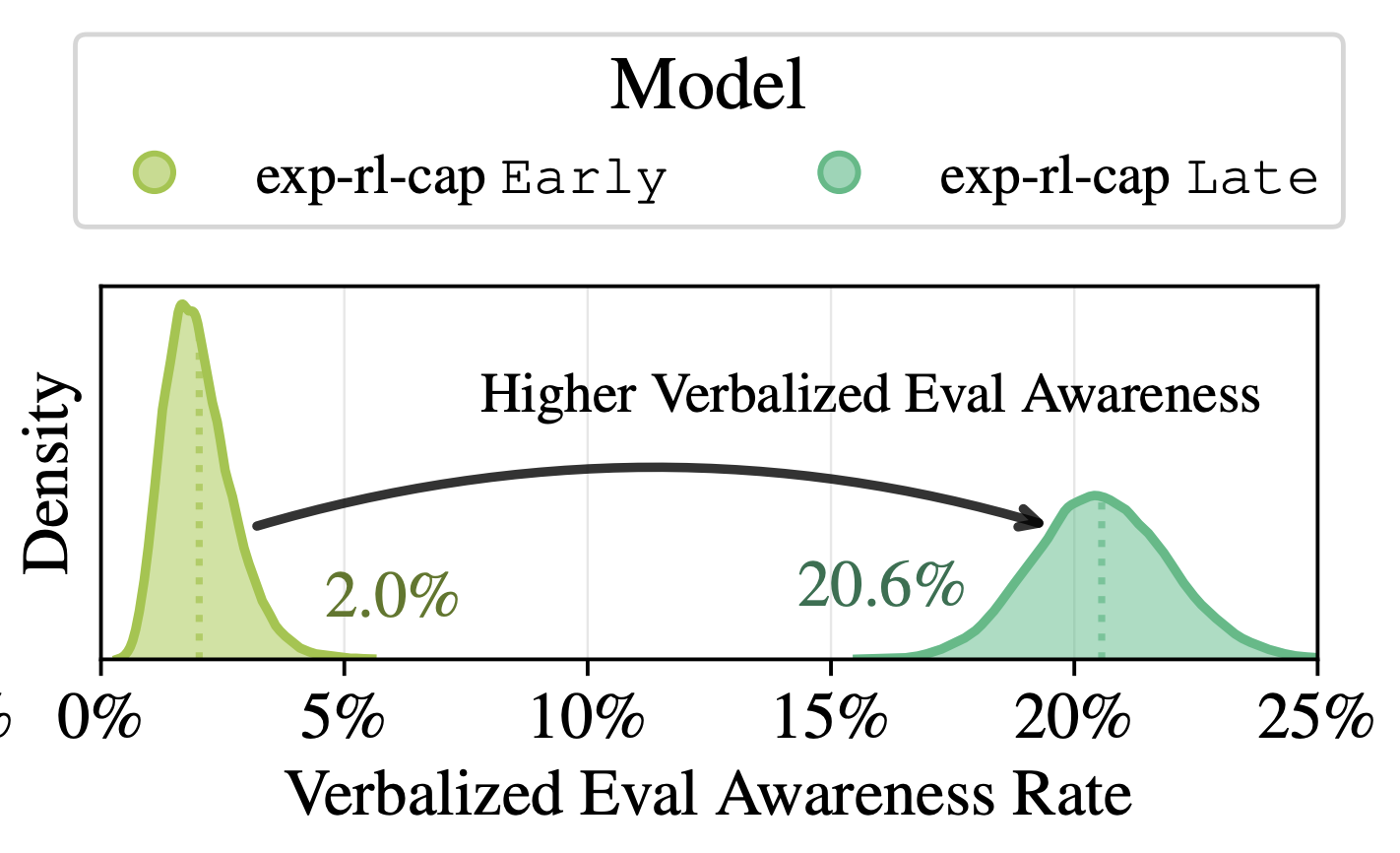
Following up on our previous work on verbalized eval awareness:we are sharing a post investigating…
Catch-Up Algorithmic Progress Might Actually be 60× per Year
Published on December 24, 2025 9:03 PM GMTEpistemic status: This is a quick analysis that…