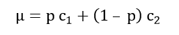
Translation from Russian. Original text available here. The first part available here.This Is a Fraud, Gentlemen!Last time we ended with a look at games where everything is fair.Well, “fair” in the sense that the chances of winning in a basic game are equal — although perhaps the very fact that they do not depend on the player’s intelligence, skill, or morality is precisely what is unfair.But let’s take a look at what happens if one of the players is so clever that he can slightly predict the coin toss. Therefore, his probability of guessing, and consequently winning, is slightly more than one-half.Or, if you prefer, a slightly asymmetrical coin is used, landing heads slightly more often, and the particularly talented player always bets on heads.In this case, the mathematical expectation of the win is no longer zero. In general — for two possible outcomes — it is calculated by the formula:Where is the probability of the first outcome, and with are the values of the outcomes.In this case, the first outcome is the first player winning, and the outcome values are winning and losing of the same amount. So in this game, the mathematical expectation of the first player’s win is…It’s easy to see that if the win probability is ½, the expectation is zero, but what happens if the probability differs from one-half?Let’s write it like this:Now, substituting this into the expectation formula gives:Let’s suppose that, instead of cleverly guessing, the talented player simply convinces his opponent that his services to society and himself absolutely require that when he guesses correctly, he receives more than he loses when he doesn’t. Say, more by . However, he will now guess and not guess with equal probability.Comparing these two results, we can conclude that a game with a higher probability of guessing is identical in terms of expected win to a game with a higher winning amount, if they are placed in the ratio:For example, if the talented player guesses with a frequency of 0.6 instead of 0.5, he could just as well stop cheating and simply demand a win of not one dollar, but…If we conduct a whole series of games with that specified probability of guessing — say, one hundred rounds — then in terms of the money in the players’ hands, we would see approximately the following.As can be seen, although the talented player even loses slightly to the other player at times, the severe bonus in guessing probability (or the increased win compared to the other player) still prevails. And over a long series of games, it will prevail in the vast majority of cases.Thus, in only about 165 games of 100 coin tosses out of 10,000 will this clever fellow lose.If the number of tosses per game increases to 1000, then the second player would be very lucky to win even once out of 10,000.Play, Come OnYou might ask: who in their right mind would play such games? If winning is only possible in a series of a few rounds, but inevitable loss occurs over a long series?Oh, you would be amazed at how many people agree to this.Take roulette, for example. If you bet on red or black, it seems the probability of winning is ½. And if you win, they return double your bet…However, roulette has a colorless zero, which makes the probability of guessing less than ½. And it’s good if there’s only one — sometimes there are two.In total, on a single-zero roulette wheel, there are 37 numbers, so the probability of winning is:The mathematical expectation of winning in a roulette game is thus:Where is the bet size.That is, in each game, on average, you give the casino one thirty-seventh of what you bet. Quite an interesting tip.Let’s play a trial series of virtual roulette games with a one-dollar bet.In this experiment, the beginning is lucky but somewhere around the two-thousandth game, the virtual player’s life clearly went downhill.”Yes, but he was winning at first, wasn’t he?” someone might say. “He could have stopped in time and left.”Indeed, you could. But only if you knew when.Moreover, besides the impossibility of knowing exactly when to leave, there is a second point: you can never return. Never.Because the process does not “reset” at the moment you leave. If this virtual player had left around the thousandth game with a $50 win, and then came again later, exactly this graph could repeat itself. And by the ten-thousandth game, he would have a total loss of $200 (from the amount he had before the first game).Furthermore, I note, this will be the case even if the casino does not cheat and the croupier does not try to land the ball in a specific spot during the throw.However, the presence of local winning streaks, visible to the naked eye on the graph, not to mention the inner feeling of “I’m on a roll today,” can mislead about the entire process and make one think that the main thing is to leave on time.Oh no, the main thing is never to return.In summary, out of a thousand people brave enough to play 10,000 roulette games with a one-dollar bet per game, about four will end up with a small win.The happiest of them will win about $70.But how much will the casino win in total?Drumroll…$273,430.Wow from WitAlright, so far I’ve considered cheating and luck, but there are other ways to win games.Clearly, the hint about roulette was meant to finally lead the reader to that very “skewed bell curve” mentioned at the end of the previous article.”Look, that distortion is supposedly caused by some players cheating.””But wait, perhaps they just play better? In that very game where profitable deals are made not by coin toss but by rational calculation, hard work, and other positive things?”Oh yes, blaming player of cheating would negate all conclusions that the observed distribution is strictly a result of luck. Blind chance, and all that. If we assume cheating, why not assume something else — like hard work and valuable skills?However, I, surprisingly, was not going to assume anything of the sort — not even cheating. On the contrary, I added this option — cheating or cleverness — only later, after I had found another option that actually yielded the desired distribution.Nevertheless, to dispel doubts about “what if this option also works?!”, let’s take a look at how the option with cheating — or, if you prefer, with intelligence and talent — would change the outcomes in the previously considered series of pairwise games. As shown in the previous sections, it can indeed manifest itself.Let me remind you of the rules. Players are randomly divided into pairs and play a coin-tossing game (now with unequal probabilities of winning) for a random bet from 1 to 10.Everyone starts with $10,000.Suppose we have 1000 players, most of whom have roughly the same skill level, but some of them still guess better.I decided to reflect this with a function of the player’s serial number — :Accordingly, for a pair of players, the probability of winning will be determined as:After everyone has played a thousand games, we get the following distribution.We already see a long “tail,” as is usually the case in real income statistics, but the main part of the bell curve is not skewed.However, here’s what the distribution of income or capital looks like in reality. Approximately like this (the numbers on the axes are conditional here).In general, it turned out somewhat similar, but not quite. There is a tail, but the “main bell” is not “skewed.”OK. Maybe we need to introduce bad players too. Let’s try this distribution of “abilities”:Alas, it got worse.Now there are two asymmetric “tails,” not at all the desired skewed bell with a “tail” on the right.Alright, we can assume that people’s abilities are distributed in a similar bell-shaped curve, which corresponds to experimental results, and use this probability of victory ratio:But even this does not yield the desired distribution: the left side, instead of “flattening,” on the contrary, stretches out.We could also try cutting off the left side of the previous option, assuming that the really stupid simply do not think to play this game and lose their money to the smart ones.Sadly, that doesn’t work either.But why?And Here Is the ReasonWe could try many more options, but the crux of the matter is that in this model, in all these experiments, we are effectively aiming for a histogram of each player’s expected win multiplied by the expected bet.Both expectations are constants for each player. Therefore, with some noise, the shapes of these histograms are predetermined from the start: the distribution of game results will resemble the distribution of abilities in shape.If we look again at the desired distribution of results……we can conclude that the first variant of the ability distribution……indeed gave something relatively close to the target.If we try to consciously adjust the ability distribution, we can use the following considerations.A player’s expected result is proportional to the ratio of his abilities to the abilities of all other players. Therefore, for a long “tail” on the right, a small group of players must have a sharp increase in abilities compared to everyone else.For the rest, abilities must grow very smoothly, according to some very intricate pattern, to provide the desired skewed bell.Somewhere at the very beginning of the graph, something else must happen to provide a decline towards complete losers — steeper than the transition from normal players to particularly talented ones.Furthermore, the result turns out to be very sensitive to the distribution of abilities, and at the slightest deviations, it immediately strongly distorts the distribution of results compared to the target.This suggests that the real process, very likely, does not depend on abilities or the ability to cheat — because if such an income distribution repeats for decades and in all countries of the world, what would ensure such high stability given such a strong dependence on the distribution of abilities?Moreover, in the left part of the distribution in the best of the found options, there is still too obvious an inflection, which in the target distribution (based on real income and personal capital distributions) is almost invisible to the naked eye.However, fine. Let’s assume that such a hypothesis has a right to exist: that is, in the world, there might indeed exist some constant proportion of mega-geniuses who win so well that the distribution of their abilities provides a long tail for the distribution of results, and some non-trivial distribution of abilities among everyone else, the cause of which is unclear.Especially since this distribution of results (called “lognormal”) is often a consequence of the presence of more than one random process in the system — what if that’s the case here too?But could there be a simpler explanation for all this, one that yields the same result without all these experimentally unverified assumptions and intricately twisted, but unobservable in studies, distributions of abilities?After all, if there are relatively simple rules of the game that provide this distribution in a fairly stable variant on their own, and something very similar to such rules is observed in reality, then it is very likely that the rules of the game themselves are the cause of the observed results, and everything else only complements them to a small extent.For example, to explain the results of “fair” pairwise coin toss, no special assumptions were needed — the rules themselves sufficed. It is possible that the same applies here.Can such rules be found?Better to Be Rich and HealthyThe ability to win more often, regardless of circumstances, is something like a “hidden parameter” in this process. But simultaneously with it, there is an “open” one: the amount of money the player currently has.Let’s assume that the probability of winning depends not on some “skills,” but simply on the amount of capital at the moment.This is a quite logical assumption: the outcome of a coin toss does not depend on the amount of money in hand, but in real transactions, it may well be that the richer person has some additional opportunities to tilt the deal in his favor. For example, bribing government agencies, hiring lobbyists in parliament, sending the mafia, or even simply benefiting from an unspoken property qualification.Suppose, for instance, that the probability of the richer player winning depends on the difference in the capitals of the two players as follows:Let’s run the previously described series of games with this probability of winning for the richer player in each pair, making the bet in each game for each pair a random number from 1 to 100.As can be seen, the hypothesis about the determining role of wealth is also not confirmed for the desired distribution: we get approximately the same symmetric bell-shaped distribution as before, which simply “spreads out” faster as the number of games played increases than it did with equal win probabilities.If we make the bet constant and higher — say, $1000 — we find that by the thousandth game, the bell curve has disappeared altogether, and the players are almost uniformly distributed according to the amounts of money they hold.That is, if implemented in reality, such a process would not give us a stable distribution of the desired shape.The rich may win more often, but some other factor is needed to explain the outcome.Dependent StakeAnother assumption we can make is that the richer can play for a higher stake. After all, the amount they are not afraid to lose is significantly higher than that of the poor.The stake is apparently determined by the player in each pair with less money, and let’s assume it is limited to one-twentieth of the money he has. However, even if the player goes deep into debt, the stake cannot be less than one dollar.And here, at some stage of the game, we finally see the desired distribution.True, by the thousandth game, the rich have almost completely fleeced most players, so the distribution becomes degenerate, “flattening” its “skewed bell” somewhere near zero.The distribution turns out to be unstable, but over a fairly long number of games it still has the desired shape.Moreover, in this experiment, along with determining the stake based on the capital of the poorer player in the pair, the same principle as in the previous section was used: the rich win more often.However, if we make winning equally probable, regardless of capital, the distribution is still maintained — only it takes more games to achieve the desired distribution and its subsequent degeneration: if by the thousandth game, with the probability of winning increasing with capital, the distribution has already degenerated, then with equal win probability, at the thousandth game, something still quite close to the desired distribution is observed.In other words, perhaps the rich do win more often, but this alone does not yield the desired distribution. On the other hand, the dependence of the stake on the current capital of the poorest player in the pair provides the desired distribution even with equal win probabilities.The same can be said about the influence of “talent” or cheating.A Small Possible ModificationI note that the variant considered here has at least one almost identical counterpart.The difference between them is only that in the original variant, each pair plays one game per round, and the stake is determined by the share of the poorest player. In the modification, however, each player per round can play several games with different players — so that the total stakes in them approximately equal a predetermined share of his capital at the beginning of the round.This modification will yield exactly the same distribution, though the processes in it will proceed somewhat faster — that is, the “tail” on the right will grow faster, and the rich will more quickly fleece the poor into poverty, if nothing is done about it. But this is mainly because the modified round includes more games with the same number of participants than the unmodified one.However, this variant is more similar to what is observed in reality, because per unit of time, the richer person can indeed participate in a larger number of low-stakes transactions than the poor person. For example, opening a store and serving a bunch of customers — also via hired employees — thus engaging in deals with both many customers and many employees.But studying such a modification is somewhat more complex for reasoning and illustration, so I will only mention that such a variant exists, and its results, simply by the very construction of the game rules, will be analogous to the results considered here.Well, after mentioning this, we can move on to the next important question.Ensuring StabilityAs mentioned two sections ago, there is one problem: this distribution turns out to be unstable and degenerates with a large number of games.If things went exactly like this in the world, the outcome of this process would be the complete impoverishment of the vast majority of players and the super-wealth of a small group of people.True, I have vague doubts: in our world, this is precisely what is observed in some places.That is, some modification of this process is needed that preserves the desired distribution even over a large number of games played.And this modification, generally speaking, is very common in reality. It is welfare benefits for the poor. They are what save particularly unlucky players from complete ruin and prevent the “bell curve” from collapsing.Let’s introduce such benefits into the game process.However, if we introduce them as a fixed amount for all time, it will only slightly delay the degeneration of the income distribution.To achieve stability, the benefit amount must depend on the current situation, and to calculate it, we will take a fairly simple maneuver.Find the largest current capital for a certain proportion of players, which will be denoted as , where is the corresponding proportion.Define the benefit amount as:It will be paid to the two-tenths of the poorest players, which should shift them approximately to where the players in the third left tenth are currently located (the graph shows only the poorest 400 out of 1000 players — otherwise, it would be difficult to see the essence of what happened).It turns out that this simplest modification is enough to maintain the stability of the distribution indefinitely.Here are the results after the six-hundredth game.After the thousandth.After the three-thousandth.It can be seen that as the number of games increases, the “tail” of the distribution stretches, but the shape itself, similar to the desired one, is preserved.Finally, thanks to benefits apparently based on printing money, inflation clearly occurs. Starting with $10,000 per person, after three thousand games, we have reached a state where even the poor have nine-figure capitals.However, inflation can be eliminated: instead of printing new money, we can introduce “taxes” from which benefits will be paid.After each round, a certain percentage of each player’s current capital will be collected, which will then be immediately distributed evenly among those in need. This percentage will be determined at each stage so that the total tax from all players fully covers all benefits paid.Now, as can be seen, bliss has arrived: the distribution is exactly what is needed, it is stable as the number of games played increases, and there is no inflation.I even tried conducting ten thousand games for ten thousand players, instead of a thousand for a thousand, and making the stake one-fifth of the capital of the poorest in the pair, instead of one-twentieth. And everything still worked out.Compare with the most successful variant of simulating the desired distribution using talent or cheating.And with the desired — “classical” lognormal distribution itself.A Suspicious ModelJust in case, I will describe the essence of the process once more.A group of players, possessing absolutely equal initial capital, is randomly divided into pairs, and then in each pair, the players play one game of coin toss.The coin toss is completely fair, so each player’s win in the pair is equally probable.The stake in each game of each pair is determined by a certain share of the current capital in the hands of the poorest player in that pair.After the game, the poorest two-tenths of players receive benefits collected from all players in the form of a percentage of their current capital, such that the total collected covers the benefits paid.After that, the players are randomly divided into pairs again and play coin toss again.As a result, we obtain a lognormal distribution of capitals — in the form of a left-skewed “bell curve” with a tail. This distribution is quite stable — with the caveat that the tail continues to lengthen as the number of games played increases (and indeed, a similar phenomenon occurs in the real world).Nothing depends on the intelligence or talents of the players.Only the size of the bet depends on capital.But, surprisingly, the distribution obtained in this game replicates the one that is actually observed in the distribution of people’s capitals (and incomes).The determining rule of the game turns out to be the quite rational and expected dependence of the stake on the capitals of each player in each pair. With this rule, it is possible to reproduce the distribution (and the observed in reality process of tail lengthening), even with absolutely equal probability of winning and losing. Without it, no linking of the win probability to “talent” or current capital helps.Stabilizing the distribution is achieved through the distribution of benefits. This is also observed in reality — as is the inevitable impoverishment of the majority of citizens in the absence of benefits in one form or another.That is, this distribution is embedded in the very “rules of the game” — in the very way the “players” interact.And indeed, primarily in the rules themselves.A player’s talent, which increases the probability of winning, or the ability to use capital to pressure the situation and similarly increase the probability of winning — these are just additions to the process, which perhaps accelerate it and introduce some non-essential corrections (and I checked, this is indeed the case), but are not themselves the main factors forming this distribution.With players absolutely identical in terms of their abilities and completely equal in rights and opportunities, regardless of capital, we would still observe exactly the same income distribution.The rules of a fairly simple and completely random game turn out to be more important than everything else.It is enough simply to make free commercial transactions, where it is equally probable to win or lose an amount that both partners consider acceptable to lose, and to pay benefits to those who lose particularly heavily.And that’s it. It will be roughly what exists now. Everywhere.However, these rules of the game are not the only ones. I have another version of the game that yields similar results. Perhaps, at least in it, we will be able to observe the determining role of talents?Spoiler: no.But that will be in the next part.Discuss Read More
Counterintuitive Coin Toss. Part II
Translation from Russian. Original text available here. The first part available here.This Is a Fraud, Gentlemen!Last time we ended with a look at games where everything is fair.Well, “fair” in the sense that the chances of winning in a basic game are equal — although perhaps the very fact that they do not depend on the player’s intelligence, skill, or morality is precisely what is unfair.But let’s take a look at what happens if one of the players is so clever that he can slightly predict the coin toss. Therefore, his probability of guessing, and consequently winning, is slightly more than one-half.Or, if you prefer, a slightly asymmetrical coin is used, landing heads slightly more often, and the particularly talented player always bets on heads.In this case, the mathematical expectation of the win is no longer zero. In general — for two possible outcomes — it is calculated by the formula:Where is the probability of the first outcome, and with are the values of the outcomes.In this case, the first outcome is the first player winning, and the outcome values are winning and losing of the same amount. So in this game, the mathematical expectation of the first player’s win is…It’s easy to see that if the win probability is ½, the expectation is zero, but what happens if the probability differs from one-half?Let’s write it like this:Now, substituting this into the expectation formula gives:Let’s suppose that, instead of cleverly guessing, the talented player simply convinces his opponent that his services to society and himself absolutely require that when he guesses correctly, he receives more than he loses when he doesn’t. Say, more by . However, he will now guess and not guess with equal probability.Comparing these two results, we can conclude that a game with a higher probability of guessing is identical in terms of expected win to a game with a higher winning amount, if they are placed in the ratio:For example, if the talented player guesses with a frequency of 0.6 instead of 0.5, he could just as well stop cheating and simply demand a win of not one dollar, but…If we conduct a whole series of games with that specified probability of guessing — say, one hundred rounds — then in terms of the money in the players’ hands, we would see approximately the following.As can be seen, although the talented player even loses slightly to the other player at times, the severe bonus in guessing probability (or the increased win compared to the other player) still prevails. And over a long series of games, it will prevail in the vast majority of cases.Thus, in only about 165 games of 100 coin tosses out of 10,000 will this clever fellow lose.If the number of tosses per game increases to 1000, then the second player would be very lucky to win even once out of 10,000.Play, Come OnYou might ask: who in their right mind would play such games? If winning is only possible in a series of a few rounds, but inevitable loss occurs over a long series?Oh, you would be amazed at how many people agree to this.Take roulette, for example. If you bet on red or black, it seems the probability of winning is ½. And if you win, they return double your bet…However, roulette has a colorless zero, which makes the probability of guessing less than ½. And it’s good if there’s only one — sometimes there are two.In total, on a single-zero roulette wheel, there are 37 numbers, so the probability of winning is:The mathematical expectation of winning in a roulette game is thus:Where is the bet size.That is, in each game, on average, you give the casino one thirty-seventh of what you bet. Quite an interesting tip.Let’s play a trial series of virtual roulette games with a one-dollar bet.In this experiment, the beginning is lucky but somewhere around the two-thousandth game, the virtual player’s life clearly went downhill.”Yes, but he was winning at first, wasn’t he?” someone might say. “He could have stopped in time and left.”Indeed, you could. But only if you knew when.Moreover, besides the impossibility of knowing exactly when to leave, there is a second point: you can never return. Never.Because the process does not “reset” at the moment you leave. If this virtual player had left around the thousandth game with a $50 win, and then came again later, exactly this graph could repeat itself. And by the ten-thousandth game, he would have a total loss of $200 (from the amount he had before the first game).Furthermore, I note, this will be the case even if the casino does not cheat and the croupier does not try to land the ball in a specific spot during the throw.However, the presence of local winning streaks, visible to the naked eye on the graph, not to mention the inner feeling of “I’m on a roll today,” can mislead about the entire process and make one think that the main thing is to leave on time.Oh no, the main thing is never to return.In summary, out of a thousand people brave enough to play 10,000 roulette games with a one-dollar bet per game, about four will end up with a small win.The happiest of them will win about $70.But how much will the casino win in total?Drumroll…$273,430.Wow from WitAlright, so far I’ve considered cheating and luck, but there are other ways to win games.Clearly, the hint about roulette was meant to finally lead the reader to that very “skewed bell curve” mentioned at the end of the previous article.”Look, that distortion is supposedly caused by some players cheating.””But wait, perhaps they just play better? In that very game where profitable deals are made not by coin toss but by rational calculation, hard work, and other positive things?”Oh yes, blaming player of cheating would negate all conclusions that the observed distribution is strictly a result of luck. Blind chance, and all that. If we assume cheating, why not assume something else — like hard work and valuable skills?However, I, surprisingly, was not going to assume anything of the sort — not even cheating. On the contrary, I added this option — cheating or cleverness — only later, after I had found another option that actually yielded the desired distribution.Nevertheless, to dispel doubts about “what if this option also works?!”, let’s take a look at how the option with cheating — or, if you prefer, with intelligence and talent — would change the outcomes in the previously considered series of pairwise games. As shown in the previous sections, it can indeed manifest itself.Let me remind you of the rules. Players are randomly divided into pairs and play a coin-tossing game (now with unequal probabilities of winning) for a random bet from 1 to 10.Everyone starts with $10,000.Suppose we have 1000 players, most of whom have roughly the same skill level, but some of them still guess better.I decided to reflect this with a function of the player’s serial number — :Accordingly, for a pair of players, the probability of winning will be determined as:After everyone has played a thousand games, we get the following distribution.We already see a long “tail,” as is usually the case in real income statistics, but the main part of the bell curve is not skewed.However, here’s what the distribution of income or capital looks like in reality. Approximately like this (the numbers on the axes are conditional here).In general, it turned out somewhat similar, but not quite. There is a tail, but the “main bell” is not “skewed.”OK. Maybe we need to introduce bad players too. Let’s try this distribution of “abilities”:Alas, it got worse.Now there are two asymmetric “tails,” not at all the desired skewed bell with a “tail” on the right.Alright, we can assume that people’s abilities are distributed in a similar bell-shaped curve, which corresponds to experimental results, and use this probability of victory ratio:But even this does not yield the desired distribution: the left side, instead of “flattening,” on the contrary, stretches out.We could also try cutting off the left side of the previous option, assuming that the really stupid simply do not think to play this game and lose their money to the smart ones.Sadly, that doesn’t work either.But why?And Here Is the ReasonWe could try many more options, but the crux of the matter is that in this model, in all these experiments, we are effectively aiming for a histogram of each player’s expected win multiplied by the expected bet.Both expectations are constants for each player. Therefore, with some noise, the shapes of these histograms are predetermined from the start: the distribution of game results will resemble the distribution of abilities in shape.If we look again at the desired distribution of results……we can conclude that the first variant of the ability distribution……indeed gave something relatively close to the target.If we try to consciously adjust the ability distribution, we can use the following considerations.A player’s expected result is proportional to the ratio of his abilities to the abilities of all other players. Therefore, for a long “tail” on the right, a small group of players must have a sharp increase in abilities compared to everyone else.For the rest, abilities must grow very smoothly, according to some very intricate pattern, to provide the desired skewed bell.Somewhere at the very beginning of the graph, something else must happen to provide a decline towards complete losers — steeper than the transition from normal players to particularly talented ones.Furthermore, the result turns out to be very sensitive to the distribution of abilities, and at the slightest deviations, it immediately strongly distorts the distribution of results compared to the target.This suggests that the real process, very likely, does not depend on abilities or the ability to cheat — because if such an income distribution repeats for decades and in all countries of the world, what would ensure such high stability given such a strong dependence on the distribution of abilities?Moreover, in the left part of the distribution in the best of the found options, there is still too obvious an inflection, which in the target distribution (based on real income and personal capital distributions) is almost invisible to the naked eye.However, fine. Let’s assume that such a hypothesis has a right to exist: that is, in the world, there might indeed exist some constant proportion of mega-geniuses who win so well that the distribution of their abilities provides a long tail for the distribution of results, and some non-trivial distribution of abilities among everyone else, the cause of which is unclear.Especially since this distribution of results (called “lognormal”) is often a consequence of the presence of more than one random process in the system — what if that’s the case here too?But could there be a simpler explanation for all this, one that yields the same result without all these experimentally unverified assumptions and intricately twisted, but unobservable in studies, distributions of abilities?After all, if there are relatively simple rules of the game that provide this distribution in a fairly stable variant on their own, and something very similar to such rules is observed in reality, then it is very likely that the rules of the game themselves are the cause of the observed results, and everything else only complements them to a small extent.For example, to explain the results of “fair” pairwise coin toss, no special assumptions were needed — the rules themselves sufficed. It is possible that the same applies here.Can such rules be found?Better to Be Rich and HealthyThe ability to win more often, regardless of circumstances, is something like a “hidden parameter” in this process. But simultaneously with it, there is an “open” one: the amount of money the player currently has.Let’s assume that the probability of winning depends not on some “skills,” but simply on the amount of capital at the moment.This is a quite logical assumption: the outcome of a coin toss does not depend on the amount of money in hand, but in real transactions, it may well be that the richer person has some additional opportunities to tilt the deal in his favor. For example, bribing government agencies, hiring lobbyists in parliament, sending the mafia, or even simply benefiting from an unspoken property qualification.Suppose, for instance, that the probability of the richer player winning depends on the difference in the capitals of the two players as follows:Let’s run the previously described series of games with this probability of winning for the richer player in each pair, making the bet in each game for each pair a random number from 1 to 100.As can be seen, the hypothesis about the determining role of wealth is also not confirmed for the desired distribution: we get approximately the same symmetric bell-shaped distribution as before, which simply “spreads out” faster as the number of games played increases than it did with equal win probabilities.If we make the bet constant and higher — say, $1000 — we find that by the thousandth game, the bell curve has disappeared altogether, and the players are almost uniformly distributed according to the amounts of money they hold.That is, if implemented in reality, such a process would not give us a stable distribution of the desired shape.The rich may win more often, but some other factor is needed to explain the outcome.Dependent StakeAnother assumption we can make is that the richer can play for a higher stake. After all, the amount they are not afraid to lose is significantly higher than that of the poor.The stake is apparently determined by the player in each pair with less money, and let’s assume it is limited to one-twentieth of the money he has. However, even if the player goes deep into debt, the stake cannot be less than one dollar.And here, at some stage of the game, we finally see the desired distribution.True, by the thousandth game, the rich have almost completely fleeced most players, so the distribution becomes degenerate, “flattening” its “skewed bell” somewhere near zero.The distribution turns out to be unstable, but over a fairly long number of games it still has the desired shape.Moreover, in this experiment, along with determining the stake based on the capital of the poorer player in the pair, the same principle as in the previous section was used: the rich win more often.However, if we make winning equally probable, regardless of capital, the distribution is still maintained — only it takes more games to achieve the desired distribution and its subsequent degeneration: if by the thousandth game, with the probability of winning increasing with capital, the distribution has already degenerated, then with equal win probability, at the thousandth game, something still quite close to the desired distribution is observed.In other words, perhaps the rich do win more often, but this alone does not yield the desired distribution. On the other hand, the dependence of the stake on the current capital of the poorest player in the pair provides the desired distribution even with equal win probabilities.The same can be said about the influence of “talent” or cheating.A Small Possible ModificationI note that the variant considered here has at least one almost identical counterpart.The difference between them is only that in the original variant, each pair plays one game per round, and the stake is determined by the share of the poorest player. In the modification, however, each player per round can play several games with different players — so that the total stakes in them approximately equal a predetermined share of his capital at the beginning of the round.This modification will yield exactly the same distribution, though the processes in it will proceed somewhat faster — that is, the “tail” on the right will grow faster, and the rich will more quickly fleece the poor into poverty, if nothing is done about it. But this is mainly because the modified round includes more games with the same number of participants than the unmodified one.However, this variant is more similar to what is observed in reality, because per unit of time, the richer person can indeed participate in a larger number of low-stakes transactions than the poor person. For example, opening a store and serving a bunch of customers — also via hired employees — thus engaging in deals with both many customers and many employees.But studying such a modification is somewhat more complex for reasoning and illustration, so I will only mention that such a variant exists, and its results, simply by the very construction of the game rules, will be analogous to the results considered here.Well, after mentioning this, we can move on to the next important question.Ensuring StabilityAs mentioned two sections ago, there is one problem: this distribution turns out to be unstable and degenerates with a large number of games.If things went exactly like this in the world, the outcome of this process would be the complete impoverishment of the vast majority of players and the super-wealth of a small group of people.True, I have vague doubts: in our world, this is precisely what is observed in some places.That is, some modification of this process is needed that preserves the desired distribution even over a large number of games played.And this modification, generally speaking, is very common in reality. It is welfare benefits for the poor. They are what save particularly unlucky players from complete ruin and prevent the “bell curve” from collapsing.Let’s introduce such benefits into the game process.However, if we introduce them as a fixed amount for all time, it will only slightly delay the degeneration of the income distribution.To achieve stability, the benefit amount must depend on the current situation, and to calculate it, we will take a fairly simple maneuver.Find the largest current capital for a certain proportion of players, which will be denoted as , where is the corresponding proportion.Define the benefit amount as:It will be paid to the two-tenths of the poorest players, which should shift them approximately to where the players in the third left tenth are currently located (the graph shows only the poorest 400 out of 1000 players — otherwise, it would be difficult to see the essence of what happened).It turns out that this simplest modification is enough to maintain the stability of the distribution indefinitely.Here are the results after the six-hundredth game.After the thousandth.After the three-thousandth.It can be seen that as the number of games increases, the “tail” of the distribution stretches, but the shape itself, similar to the desired one, is preserved.Finally, thanks to benefits apparently based on printing money, inflation clearly occurs. Starting with $10,000 per person, after three thousand games, we have reached a state where even the poor have nine-figure capitals.However, inflation can be eliminated: instead of printing new money, we can introduce “taxes” from which benefits will be paid.After each round, a certain percentage of each player’s current capital will be collected, which will then be immediately distributed evenly among those in need. This percentage will be determined at each stage so that the total tax from all players fully covers all benefits paid.Now, as can be seen, bliss has arrived: the distribution is exactly what is needed, it is stable as the number of games played increases, and there is no inflation.I even tried conducting ten thousand games for ten thousand players, instead of a thousand for a thousand, and making the stake one-fifth of the capital of the poorest in the pair, instead of one-twentieth. And everything still worked out.Compare with the most successful variant of simulating the desired distribution using talent or cheating.And with the desired — “classical” lognormal distribution itself.A Suspicious ModelJust in case, I will describe the essence of the process once more.A group of players, possessing absolutely equal initial capital, is randomly divided into pairs, and then in each pair, the players play one game of coin toss.The coin toss is completely fair, so each player’s win in the pair is equally probable.The stake in each game of each pair is determined by a certain share of the current capital in the hands of the poorest player in that pair.After the game, the poorest two-tenths of players receive benefits collected from all players in the form of a percentage of their current capital, such that the total collected covers the benefits paid.After that, the players are randomly divided into pairs again and play coin toss again.As a result, we obtain a lognormal distribution of capitals — in the form of a left-skewed “bell curve” with a tail. This distribution is quite stable — with the caveat that the tail continues to lengthen as the number of games played increases (and indeed, a similar phenomenon occurs in the real world).Nothing depends on the intelligence or talents of the players.Only the size of the bet depends on capital.But, surprisingly, the distribution obtained in this game replicates the one that is actually observed in the distribution of people’s capitals (and incomes).The determining rule of the game turns out to be the quite rational and expected dependence of the stake on the capitals of each player in each pair. With this rule, it is possible to reproduce the distribution (and the observed in reality process of tail lengthening), even with absolutely equal probability of winning and losing. Without it, no linking of the win probability to “talent” or current capital helps.Stabilizing the distribution is achieved through the distribution of benefits. This is also observed in reality — as is the inevitable impoverishment of the majority of citizens in the absence of benefits in one form or another.That is, this distribution is embedded in the very “rules of the game” — in the very way the “players” interact.And indeed, primarily in the rules themselves.A player’s talent, which increases the probability of winning, or the ability to use capital to pressure the situation and similarly increase the probability of winning — these are just additions to the process, which perhaps accelerate it and introduce some non-essential corrections (and I checked, this is indeed the case), but are not themselves the main factors forming this distribution.With players absolutely identical in terms of their abilities and completely equal in rights and opportunities, regardless of capital, we would still observe exactly the same income distribution.The rules of a fairly simple and completely random game turn out to be more important than everything else.It is enough simply to make free commercial transactions, where it is equally probable to win or lose an amount that both partners consider acceptable to lose, and to pay benefits to those who lose particularly heavily.And that’s it. It will be roughly what exists now. Everywhere.However, these rules of the game are not the only ones. I have another version of the game that yields similar results. Perhaps, at least in it, we will be able to observe the determining role of talents?Spoiler: no.But that will be in the next part.Discuss Read More
Related Posts

Project Glasswing: Anthropic Shows The AI Train Isn’t Stopping
Note: This was initially written for a more general audience, but does contain information that…
Don’t Let LLMs Write For You
Content note: nothing in this piece is a prank or jumpscare where I smirkingly reveal…
Schedule meetings using the Pareto principle
Basically every meeting is scheduled with an explicit duration. This is convenient for scheduling, but…