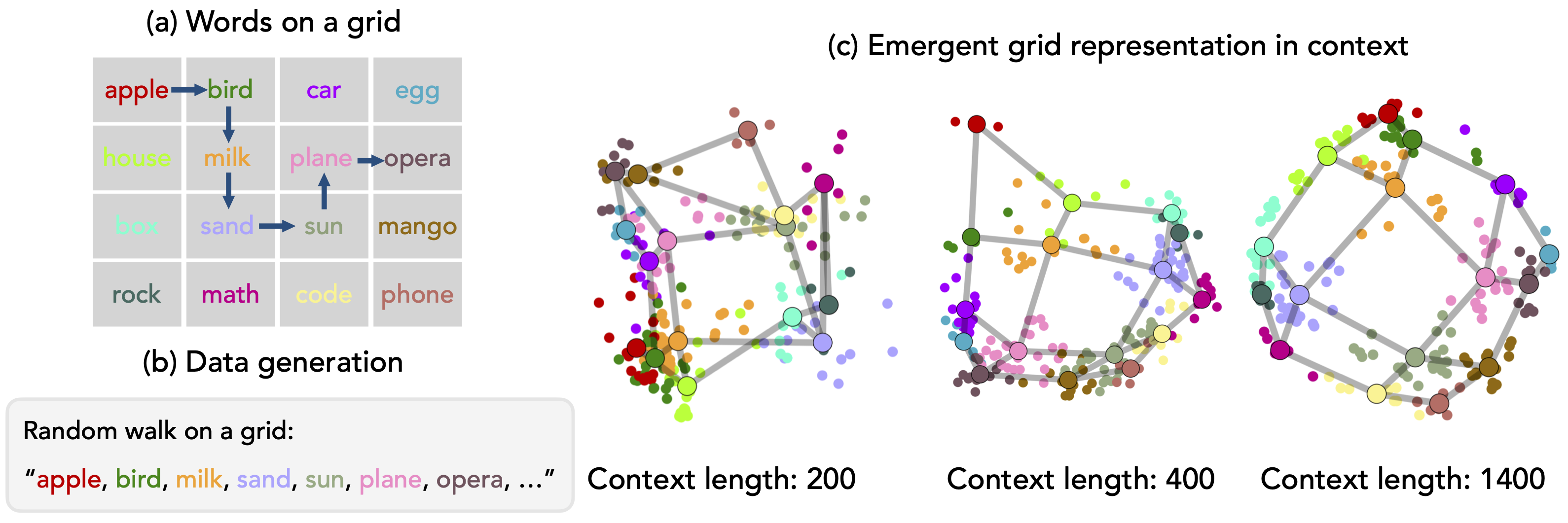
This is a crosspost of my ICLR 2026 blogpost track post. All code and experiments are available at github.com/andyrdt/iclr_induction.SummaryPark et al., 2025 show that when large language models (LLMs) process random walks on a graph, their internal representations come to mirror the underlying graph’s structure. The authors interpret this broadly, suggesting that LLMs can “manipulate their representations in order to reflect concept semantics specified entirely in-context”. In this post, we take a closer look at the underlying mechanism, and suggest a simpler explanation. We argue that induction circuits (Elhage et al., 2021; Olsson et al., 2022), a well-known mechanism for in-context bigram recall, suffice to explain both the task performance and the representation geometry observed by Park et al.Recapitulation and reproduction of Park et al., 2025We begin by describing the experimental setup of Park et al., 2025 and reproducing their main results on Llama-3.1-8B.Figure 1. Overview of Park et al.(a) The grid tracing task uses a 4×4 grid of words. (b) Models observe random walks on the grid (e.g., apple bird milk sand sun plane opera …) where consecutive words are always neighbors. As the sequence length grows, the model begins to predict valid next words based on the graph structure. (c) Surprisingly, the geometry of the model’s effective token representations mirrors that of the grid structure: the model comes to represent each node adjacent to its neighbor in activation space. Figure reproduced from Park et al.The grid tracing taskPark et al. introduce the in-context graph tracing task. The task involves a predefined graph where nodes are referenced via tokens (e.g., apple, bird, math, etc.). The graph’s connectivity structure is defined independently of any semantic relationships between the tokens. The model is provided with traces of random walks on this graph as context and must predict valid next nodes based on the learned connectivity structure. While Park et al. study graph tracing on three different graph structures, we focus exclusively on their square grid setting (Figure 1). We provide details of the experimental setup below; our methodology always follows Park et al. except when otherwise noted.Grid structure. The task uses a grid of 16 distinct word tokens: apple, bird, car, egg, house, milk, plane, opera, box, sand, sun, mango, rock, math, code, phone.[1] Each word occupies a unique position in the grid. Two words are neighbors if they are horizontally or vertically adjacent (not diagonally). This defines an adjacency matrix where if and only if words and are neighbors.Random walk generation. Sequences are generated by random walks on this grid: starting from a random position, the walk moves to a uniformly random neighbor at each step. This produces sequences like apple bird milk sand sun plane opera … where consecutive words are always grid neighbors. Following Park et al., we use sequence lengths of 1400 tokens.Measuring accuracy. At timestep , the walk is at node with neighbors , and the model outputs a distribution over vocabulary tokens. Following Park et al., we define “rule following accuracy” as the total probability mass assigned to valid next nodes:PCA visualization. To assess whether the model’s representations come to resemble the grid structure, we extract activations from a late layer (layer 26 out of 32). For each of the 16 words, we compute a class-mean activation by averaging over all occurrences in the final 200 positions of the sequence. We then project these 16 class-mean vectors onto their first two principal components for visualization. If the representation geometry reflects the grid, neighboring tokens should appear nearby in this projection.Reproduction and Park et al.’s interpretationFigure 2 shows our reproduction of Park et al.’s main results on Llama-3.1-8B.Figure 2. Reproduction of main results from Park et al.Left: Model accuracy on the grid tracing task increases with context length, reaching accuracy after tokens. Shaded region shows standard deviation across 16 random sequences. Right: PCA projection of class-mean activations at layer 26 after seeing 1400 tokens. Gray dashed lines connect grid neighbors. The geometry of the effective representations resembles the grid structure underlying the data.Park et al. interpret these findings as evidence that the geometric reorganization plays a functional role in task performance: the model learns the graph structure in its representations, and this learned structure is what enables accurate next-node predictions.”We see once a critical amount of context is seen by the model, accuracy starts to rapidly improve. We find this point in fact closely matches when Dirichlet energy[2] reaches its minimum value: energy is minimized shortly before the rapid increase in in-context task accuracy, suggesting that the structure of the data is correctly learned before the model can make valid predictions. This leads us to the claim that as the amount of context is scaled, there is an emergent re-organization of representations that allows the model to perform well on our in-context graph tracing task.”— Park et al. (Section 4.1; emphasis in original)A simpler explanation: induction circuitsWe propose that the grid tracing task can be solved by a much simpler mechanism than the in-context representation reorganization posited by Park et al.: induction circuits (Elhage et al., 2021; Olsson et al., 2022).An induction circuit consists of two types of attention heads working together. Previous-token heads attend from position to position , copying information about the previous token into the current position’s residual stream. Induction heads then attend to positions that follow previous occurrences of the current token. Together, they implement in-context bigram recall: “if followed before, predict when seeing again.”[3]In the grid task, if the model has seen the bigram apple bird earlier in the sequence, then upon encountering apple again, the induction circuit can retrieve and predict bird. Since consecutive tokens in a random walk are always grid neighbors, every recalled successor is guaranteed to be a valid next step. With enough context, the model will have observed multiple successors for each token, and can aggregate over these to assign probability mass to all valid neighbors.[4]Testing the induction hypothesisIf the model relies on induction circuits to solve the task, then ablating the heads that comprise them should substantially degrade task performance. We test this via zero ablation: setting targeted attention heads’ outputs to zero and measuring the causal impact on both task accuracy and in-context representations.Head identification. Following Olsson et al., 2022, we identify induction heads and previous-token heads using attention pattern analysis on repeated sequences, and rank all 1024 heads in Llama-3.1-8B by their respective scores, yielding two ranked lists.Ablation procedure. For each head type, we ablate the top- heads for and measure impact on task accuracy and representation geometry. As a control, we ablate random heads sampled from all heads excluding the top 32 induction and top 32 previous-token heads. All accuracy curves are averaged over 16 random walk sequences (one per grid starting position). The random head control additionally averages over 4 independent sets of 32 heads.ResultsFigure 3. Effect of head ablation on task accuracy.Left: Ablating top induction heads progressively degrades accuracy, but the model still learns with context. Right: Ablating top previous-token heads causes accuracy to plateau, preventing learning even with more context. Accuracy is averaged over 16 random walk sequences. The gray lines show the effect of ablating 32 random heads, excluding top induction and prev-token heads (averaged over 4 independent head sets).Both induction heads and previous-token heads are critical to task performance. Figure 3 shows task accuracy under head ablations.Ablating the top-4 induction heads causes accuracy to drop from to , and ablating the top-32 drops accuracy all the way to . Ablating just the top-2 previous-token heads reduces accuracy to below , and ablating the top-32 previous-token heads further drops accuracy to .In contrast, ablating random heads causes only minor degradation (accuracy remains at ), suggesting that induction and previous-token heads are particularly important for task performance.While both head types are important for task performance, their ablations have qualitatively different effects on in-context learning dynamics. Ablating induction heads degrades performance, but accuracy continues to ascend as context length increases. In contrast, ablating previous-token heads causes accuracy to plateau entirely.Figure 4. Effect of head ablation on representation geometry.PCA projections of class-mean activations under different ablation conditions. Left: Ablating top-32 induction heads preserves the grid geometry. Right: Ablating top-32 previous-token heads disrupts the spatial organization. This suggests previous-token heads are necessary for the geometric structure, while induction heads are not.Ablating previous-token heads disrupts representation geometry. While both head types are important for accuracy, they seem to have different effects on representation geometry. Figure 4 shows that ablating induction heads preserves the grid-like geometric structure in PCA visualizations, as the 2D projections still resemble the spatial grid. However, ablating previous-token heads disrupts this structure, causing representations to lose their apparent spatial organization.Previous-token mixing can account for representation geometryIn the previous section, we studied task performance and argued that the model achieves high task accuracy by using induction circuits. We now study the representation geometry, and attempt to explain the grid-like PCA plots. We will argue that this structure is plausibly a byproduct of “token mixing” performed by previous-token heads.The neighbor-mixing hypothesisFigure 4 shows that ablating previous-token heads disrupts the grid structure, while ablating induction heads preserves it. This suggests that previous-token heads are somehow necessary for the geometric organization. But what mechanism could link previous-token heads to spatial structure?Previous-token heads mix information from position into position . In a random walk, the token at is always a grid neighbor of the token at . So each token’s representation gets mixed with a neighbor’s. When we compute the class mean for word , we average over all positions where appears, each of which has been mixed with whichever neighbor preceded it. Over many occurrences, is preceded by each of its neighbors roughly equally, so the class mean for roughly encodes plus an average of its neighbors.To test whether neighbor-mixing alone can create the observed geometry, we construct a minimal toy model.A toy model of previous-token mixingWe work directly in a 16-token space indexed by the grid nodes. Each node is assigned an initial random vector , sampled i.i.d. from . PCA of just the raw embeddings produces an essentially unstructured cloud: there is no visible trace of the grid.We then apply a single, “neighbor mixing” step:where denotes the set of neighbors of node .After this one step, PCA of the 16 mixed vectors recovers a clear grid: neighbors are close in the 2D projection and non-neighbors are far (Figure 5).Figure 5. One round of neighbor mixing creates grid structure from random embeddings.Left: PCA projection of 16 random Gaussian vectors shows no spatial structure. Right: After applying one neighbor-mixing step, the same embeddings exhibit clear grid organization in PCA space. Gray dashed lines connect grid neighbors.Evidence of neighbor mixing in individual model activationsThe neighbor-mixing hypothesis makes a further prediction: individual activations should reflect not just the current token, but also its predecessor.Instead of collapsing each word into a single class mean, we take the final 200 positions of a length-1400 random-walk sequence and project all 200 residual-stream vectors into the same 2D PCA space used for the class means. Each point now corresponds to a specific activation. For each point, we display bigram information: the center color indicates the current token and the border color indicates the previous token .Figure 6. Bigram-level PCA visualization.Each point represents a single position’s activation. Fill color indicates the current token; border color indicates the previous token. Points with the same current token but different previous tokens form distinct clusters, suggesting the representation encodes information about both. Star markers show token centroids.Individual activations seem to bear the fingerprint of previous-token mixing (Figure 6). For example, activations at positions where the bigram plane math occurred tend to lie between the plane and math centroids, and positions where egg math occurred tend to lie between the egg and math centroids. We see similar “in-between” behavior for all other bigrams. This is what one would expect if the representation of contains something like a mixture of “self” and “previous token” rather than depending only on the current word.LimitationsOur experiments point toward a simple explanation: the model performs in-context graph tracing via induction circuits, and the grid-like PCA geometry is a byproduct of previous-token mixing. However, our understanding remains incomplete in important ways.The toy model is a significant simplification. Our neighbor-mixing rule assumes that previous-token heads simply add the previous token’s activation to the current token’s activation . In reality, attention heads apply value and output projections: they add , where is a low-rank matrix (rank ). This projection could substantially transform the information being mixed, and notably cannot implement the identity mapping (with a single head, at least) since it is low-rank. We also model everything as a single mixing step on static vectors, whereas the actual network has many attention heads, MLP blocks, and multiple layers that repeatedly transform the residual stream.Why does the grid structure emerge late in the sequence? Previous-token heads are active from the start of the sequence, yet the grid-like PCA structure only becomes clearly visible after many tokens have been processed. If neighbor-mixing were the whole story, we might expect the geometric structure to appear earlier. Yang et al., 2025 develop a theoretical framework formalizing a graph-convolution-like process across both context and layers, that may offer a more complete account of how the geometric structure emerges.Limited to the in-context grid tracing task. Our analysis is limited to the grid random walk task from Park et al., where bigram copying suffices for next-token prediction. Lepori et al., 2026 concurrently find that on these random walk tasks, the in-context representations are largely “inert” — models encode the graph topology but struggle to deploy it for downstream spatial reasoning. However, in other settings, in-context representation changes may be more functional: Yona et al., 2025 show that in-context exemplars can functionally override a token’s semantic meaning. It would also be interesting to investigate more complex in-context learning tasks where induction circuits are not sufficient, such as those with hierarchical or context-dependent structure (Saanum et al., 2025).ConclusionWe have argued that the phenomena observed by Park et al., 2025 can be explained by well-known mechanisms in language models. Task performance on in-context graph tracing is well-explained by induction circuits, which recall previously-seen bigrams. The geometric organization visible in PCA plots appears to be a byproduct of previous-token mixing: because random walks traverse graph edges, previous-token heads mix each position’s representation with that of a graph neighbor, and this mixing alone is sufficient to produce grid-like structure from unstructured embeddings.These findings suggest that the “representation reorganization” observed by Park et al. may not reflect a sophisticated in-context learning strategy, but rather an artifact of previous-token head behavior. ^All words tokenize to exactly one token when preceded by a space (e.g., apple is a single token). Sequences are tokenized with a leading space before the first word, ensuring single-token-per-word encoding.^Dirichlet energy measures how much a signal varies across graph edges. Low energy means neighboring nodes have similar representations, so Park et al. use it to quantify how well the model’s representations respect the graph structure.^In the literature, the term “induction head” is sometimes used to refer to both the individual attention head and the full two-component circuit. We use “induction circuit” for the full mechanism and “induction head” for the specific head that attends to tokens following previous occurrences, to avoid ambiguity.^For example, if the model has seen both apple bird and apple house, it can distribute probability across both bird and house when predicting the next token after apple.Discuss Read More
In-context learning of representations can be explained by induction circuits
This is a crosspost of my ICLR 2026 blogpost track post. All code and experiments are available at github.com/andyrdt/iclr_induction.SummaryPark et al., 2025 show that when large language models (LLMs) process random walks on a graph, their internal representations come to mirror the underlying graph’s structure. The authors interpret this broadly, suggesting that LLMs can “manipulate their representations in order to reflect concept semantics specified entirely in-context”. In this post, we take a closer look at the underlying mechanism, and suggest a simpler explanation. We argue that induction circuits (Elhage et al., 2021; Olsson et al., 2022), a well-known mechanism for in-context bigram recall, suffice to explain both the task performance and the representation geometry observed by Park et al.Recapitulation and reproduction of Park et al., 2025We begin by describing the experimental setup of Park et al., 2025 and reproducing their main results on Llama-3.1-8B.Figure 1. Overview of Park et al.(a) The grid tracing task uses a 4×4 grid of words. (b) Models observe random walks on the grid (e.g., apple bird milk sand sun plane opera …) where consecutive words are always neighbors. As the sequence length grows, the model begins to predict valid next words based on the graph structure. (c) Surprisingly, the geometry of the model’s effective token representations mirrors that of the grid structure: the model comes to represent each node adjacent to its neighbor in activation space. Figure reproduced from Park et al.The grid tracing taskPark et al. introduce the in-context graph tracing task. The task involves a predefined graph where nodes are referenced via tokens (e.g., apple, bird, math, etc.). The graph’s connectivity structure is defined independently of any semantic relationships between the tokens. The model is provided with traces of random walks on this graph as context and must predict valid next nodes based on the learned connectivity structure. While Park et al. study graph tracing on three different graph structures, we focus exclusively on their square grid setting (Figure 1). We provide details of the experimental setup below; our methodology always follows Park et al. except when otherwise noted.Grid structure. The task uses a grid of 16 distinct word tokens: apple, bird, car, egg, house, milk, plane, opera, box, sand, sun, mango, rock, math, code, phone.[1] Each word occupies a unique position in the grid. Two words are neighbors if they are horizontally or vertically adjacent (not diagonally). This defines an adjacency matrix where if and only if words and are neighbors.Random walk generation. Sequences are generated by random walks on this grid: starting from a random position, the walk moves to a uniformly random neighbor at each step. This produces sequences like apple bird milk sand sun plane opera … where consecutive words are always grid neighbors. Following Park et al., we use sequence lengths of 1400 tokens.Measuring accuracy. At timestep , the walk is at node with neighbors , and the model outputs a distribution over vocabulary tokens. Following Park et al., we define “rule following accuracy” as the total probability mass assigned to valid next nodes:PCA visualization. To assess whether the model’s representations come to resemble the grid structure, we extract activations from a late layer (layer 26 out of 32). For each of the 16 words, we compute a class-mean activation by averaging over all occurrences in the final 200 positions of the sequence. We then project these 16 class-mean vectors onto their first two principal components for visualization. If the representation geometry reflects the grid, neighboring tokens should appear nearby in this projection.Reproduction and Park et al.’s interpretationFigure 2 shows our reproduction of Park et al.’s main results on Llama-3.1-8B.Figure 2. Reproduction of main results from Park et al.Left: Model accuracy on the grid tracing task increases with context length, reaching accuracy after tokens. Shaded region shows standard deviation across 16 random sequences. Right: PCA projection of class-mean activations at layer 26 after seeing 1400 tokens. Gray dashed lines connect grid neighbors. The geometry of the effective representations resembles the grid structure underlying the data.Park et al. interpret these findings as evidence that the geometric reorganization plays a functional role in task performance: the model learns the graph structure in its representations, and this learned structure is what enables accurate next-node predictions.”We see once a critical amount of context is seen by the model, accuracy starts to rapidly improve. We find this point in fact closely matches when Dirichlet energy[2] reaches its minimum value: energy is minimized shortly before the rapid increase in in-context task accuracy, suggesting that the structure of the data is correctly learned before the model can make valid predictions. This leads us to the claim that as the amount of context is scaled, there is an emergent re-organization of representations that allows the model to perform well on our in-context graph tracing task.”— Park et al. (Section 4.1; emphasis in original)A simpler explanation: induction circuitsWe propose that the grid tracing task can be solved by a much simpler mechanism than the in-context representation reorganization posited by Park et al.: induction circuits (Elhage et al., 2021; Olsson et al., 2022).An induction circuit consists of two types of attention heads working together. Previous-token heads attend from position to position , copying information about the previous token into the current position’s residual stream. Induction heads then attend to positions that follow previous occurrences of the current token. Together, they implement in-context bigram recall: “if followed before, predict when seeing again.”[3]In the grid task, if the model has seen the bigram apple bird earlier in the sequence, then upon encountering apple again, the induction circuit can retrieve and predict bird. Since consecutive tokens in a random walk are always grid neighbors, every recalled successor is guaranteed to be a valid next step. With enough context, the model will have observed multiple successors for each token, and can aggregate over these to assign probability mass to all valid neighbors.[4]Testing the induction hypothesisIf the model relies on induction circuits to solve the task, then ablating the heads that comprise them should substantially degrade task performance. We test this via zero ablation: setting targeted attention heads’ outputs to zero and measuring the causal impact on both task accuracy and in-context representations.Head identification. Following Olsson et al., 2022, we identify induction heads and previous-token heads using attention pattern analysis on repeated sequences, and rank all 1024 heads in Llama-3.1-8B by their respective scores, yielding two ranked lists.Ablation procedure. For each head type, we ablate the top- heads for and measure impact on task accuracy and representation geometry. As a control, we ablate random heads sampled from all heads excluding the top 32 induction and top 32 previous-token heads. All accuracy curves are averaged over 16 random walk sequences (one per grid starting position). The random head control additionally averages over 4 independent sets of 32 heads.ResultsFigure 3. Effect of head ablation on task accuracy.Left: Ablating top induction heads progressively degrades accuracy, but the model still learns with context. Right: Ablating top previous-token heads causes accuracy to plateau, preventing learning even with more context. Accuracy is averaged over 16 random walk sequences. The gray lines show the effect of ablating 32 random heads, excluding top induction and prev-token heads (averaged over 4 independent head sets).Both induction heads and previous-token heads are critical to task performance. Figure 3 shows task accuracy under head ablations.Ablating the top-4 induction heads causes accuracy to drop from to , and ablating the top-32 drops accuracy all the way to . Ablating just the top-2 previous-token heads reduces accuracy to below , and ablating the top-32 previous-token heads further drops accuracy to .In contrast, ablating random heads causes only minor degradation (accuracy remains at ), suggesting that induction and previous-token heads are particularly important for task performance.While both head types are important for task performance, their ablations have qualitatively different effects on in-context learning dynamics. Ablating induction heads degrades performance, but accuracy continues to ascend as context length increases. In contrast, ablating previous-token heads causes accuracy to plateau entirely.Figure 4. Effect of head ablation on representation geometry.PCA projections of class-mean activations under different ablation conditions. Left: Ablating top-32 induction heads preserves the grid geometry. Right: Ablating top-32 previous-token heads disrupts the spatial organization. This suggests previous-token heads are necessary for the geometric structure, while induction heads are not.Ablating previous-token heads disrupts representation geometry. While both head types are important for accuracy, they seem to have different effects on representation geometry. Figure 4 shows that ablating induction heads preserves the grid-like geometric structure in PCA visualizations, as the 2D projections still resemble the spatial grid. However, ablating previous-token heads disrupts this structure, causing representations to lose their apparent spatial organization.Previous-token mixing can account for representation geometryIn the previous section, we studied task performance and argued that the model achieves high task accuracy by using induction circuits. We now study the representation geometry, and attempt to explain the grid-like PCA plots. We will argue that this structure is plausibly a byproduct of “token mixing” performed by previous-token heads.The neighbor-mixing hypothesisFigure 4 shows that ablating previous-token heads disrupts the grid structure, while ablating induction heads preserves it. This suggests that previous-token heads are somehow necessary for the geometric organization. But what mechanism could link previous-token heads to spatial structure?Previous-token heads mix information from position into position . In a random walk, the token at is always a grid neighbor of the token at . So each token’s representation gets mixed with a neighbor’s. When we compute the class mean for word , we average over all positions where appears, each of which has been mixed with whichever neighbor preceded it. Over many occurrences, is preceded by each of its neighbors roughly equally, so the class mean for roughly encodes plus an average of its neighbors.To test whether neighbor-mixing alone can create the observed geometry, we construct a minimal toy model.A toy model of previous-token mixingWe work directly in a 16-token space indexed by the grid nodes. Each node is assigned an initial random vector , sampled i.i.d. from . PCA of just the raw embeddings produces an essentially unstructured cloud: there is no visible trace of the grid.We then apply a single, “neighbor mixing” step:where denotes the set of neighbors of node .After this one step, PCA of the 16 mixed vectors recovers a clear grid: neighbors are close in the 2D projection and non-neighbors are far (Figure 5).Figure 5. One round of neighbor mixing creates grid structure from random embeddings.Left: PCA projection of 16 random Gaussian vectors shows no spatial structure. Right: After applying one neighbor-mixing step, the same embeddings exhibit clear grid organization in PCA space. Gray dashed lines connect grid neighbors.Evidence of neighbor mixing in individual model activationsThe neighbor-mixing hypothesis makes a further prediction: individual activations should reflect not just the current token, but also its predecessor.Instead of collapsing each word into a single class mean, we take the final 200 positions of a length-1400 random-walk sequence and project all 200 residual-stream vectors into the same 2D PCA space used for the class means. Each point now corresponds to a specific activation. For each point, we display bigram information: the center color indicates the current token and the border color indicates the previous token .Figure 6. Bigram-level PCA visualization.Each point represents a single position’s activation. Fill color indicates the current token; border color indicates the previous token. Points with the same current token but different previous tokens form distinct clusters, suggesting the representation encodes information about both. Star markers show token centroids.Individual activations seem to bear the fingerprint of previous-token mixing (Figure 6). For example, activations at positions where the bigram plane math occurred tend to lie between the plane and math centroids, and positions where egg math occurred tend to lie between the egg and math centroids. We see similar “in-between” behavior for all other bigrams. This is what one would expect if the representation of contains something like a mixture of “self” and “previous token” rather than depending only on the current word.LimitationsOur experiments point toward a simple explanation: the model performs in-context graph tracing via induction circuits, and the grid-like PCA geometry is a byproduct of previous-token mixing. However, our understanding remains incomplete in important ways.The toy model is a significant simplification. Our neighbor-mixing rule assumes that previous-token heads simply add the previous token’s activation to the current token’s activation . In reality, attention heads apply value and output projections: they add , where is a low-rank matrix (rank ). This projection could substantially transform the information being mixed, and notably cannot implement the identity mapping (with a single head, at least) since it is low-rank. We also model everything as a single mixing step on static vectors, whereas the actual network has many attention heads, MLP blocks, and multiple layers that repeatedly transform the residual stream.Why does the grid structure emerge late in the sequence? Previous-token heads are active from the start of the sequence, yet the grid-like PCA structure only becomes clearly visible after many tokens have been processed. If neighbor-mixing were the whole story, we might expect the geometric structure to appear earlier. Yang et al., 2025 develop a theoretical framework formalizing a graph-convolution-like process across both context and layers, that may offer a more complete account of how the geometric structure emerges.Limited to the in-context grid tracing task. Our analysis is limited to the grid random walk task from Park et al., where bigram copying suffices for next-token prediction. Lepori et al., 2026 concurrently find that on these random walk tasks, the in-context representations are largely “inert” — models encode the graph topology but struggle to deploy it for downstream spatial reasoning. However, in other settings, in-context representation changes may be more functional: Yona et al., 2025 show that in-context exemplars can functionally override a token’s semantic meaning. It would also be interesting to investigate more complex in-context learning tasks where induction circuits are not sufficient, such as those with hierarchical or context-dependent structure (Saanum et al., 2025).ConclusionWe have argued that the phenomena observed by Park et al., 2025 can be explained by well-known mechanisms in language models. Task performance on in-context graph tracing is well-explained by induction circuits, which recall previously-seen bigrams. The geometric organization visible in PCA plots appears to be a byproduct of previous-token mixing: because random walks traverse graph edges, previous-token heads mix each position’s representation with that of a graph neighbor, and this mixing alone is sufficient to produce grid-like structure from unstructured embeddings.These findings suggest that the “representation reorganization” observed by Park et al. may not reflect a sophisticated in-context learning strategy, but rather an artifact of previous-token head behavior. ^All words tokenize to exactly one token when preceded by a space (e.g., apple is a single token). Sequences are tokenized with a leading space before the first word, ensuring single-token-per-word encoding.^Dirichlet energy measures how much a signal varies across graph edges. Low energy means neighboring nodes have similar representations, so Park et al. use it to quantify how well the model’s representations respect the graph structure.^In the literature, the term “induction head” is sometimes used to refer to both the individual attention head and the full two-component circuit. We use “induction circuit” for the full mechanism and “induction head” for the specific head that attends to tokens following previous occurrences, to avoid ambiguity.^For example, if the model has seen both apple bird and apple house, it can distribute probability across both bird and house when predicting the next token after apple.Discuss Read More
Related Posts

‘Safe by Design’: A Speculative Paradigm for Positive AI Development
Published on November 28, 2025 3:04 PM GMTStatus: These were some rough ideas I was…
Evolution & Freedom
Published on November 26, 2025 3:38 AM GMTIn Against Money Maximalism, I argued against money-maximization…
$500 Write like lsusr competition – Results
Published on January 1, 2026 8:53 PM GMTHere are the results of our New Year…